Glyphs, Streamlines, Stream Tubes, Stream Surfaces
Part 1: Glyphs for Visualizing the Vector Field The first task is to visualize the velocity of the flow using glyphs (cones, cylinders, and arrows). We use a cutting plane orthogonal to the x-axis and position it at three different locations. We coded the magnitude velocities to {25 -> blue, 50 -> cyan, 75 -> green, 100 -> pink, 125 -> red}. We also scale the glyphs by the magnitude. The color transfer function is used in the other visualizations as well. We tried positioning the plane in various locations. Among those we found the three locations (40,0,0), (70,0,0), (150,0,0) to be the most interesting. However, we have also found the locations (30,0,0), (200,0,0), (300,0,0), (110,0,0) to be interesting and include renderings of these features as well. |
Part 1.1: Cone Glyphs The four images below are rendered at location (40,0,0). 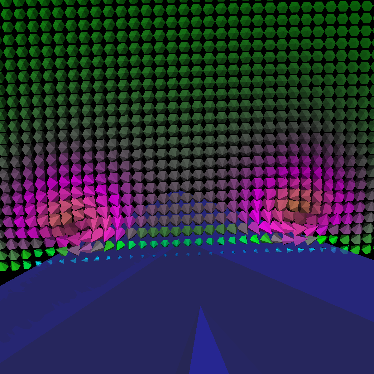 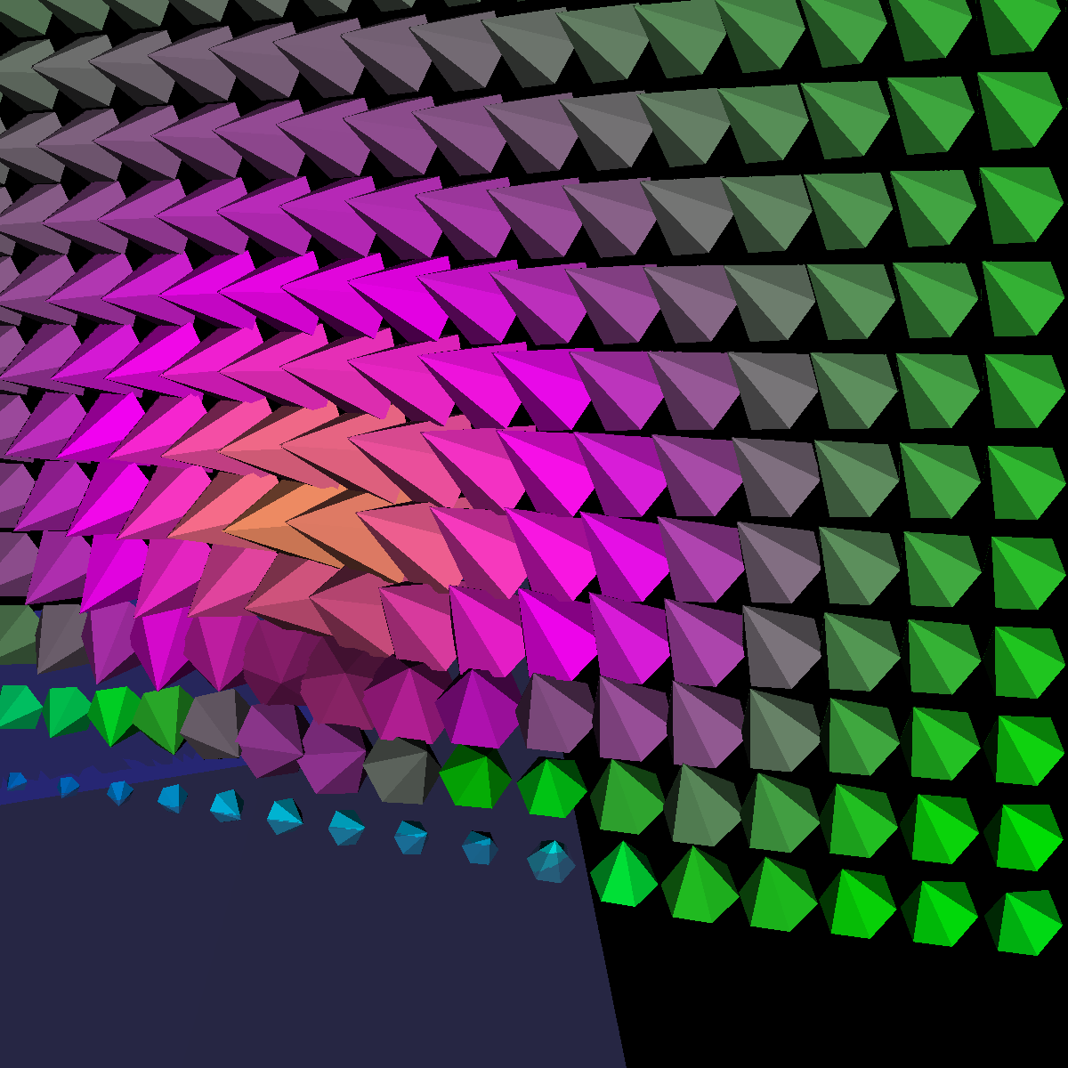 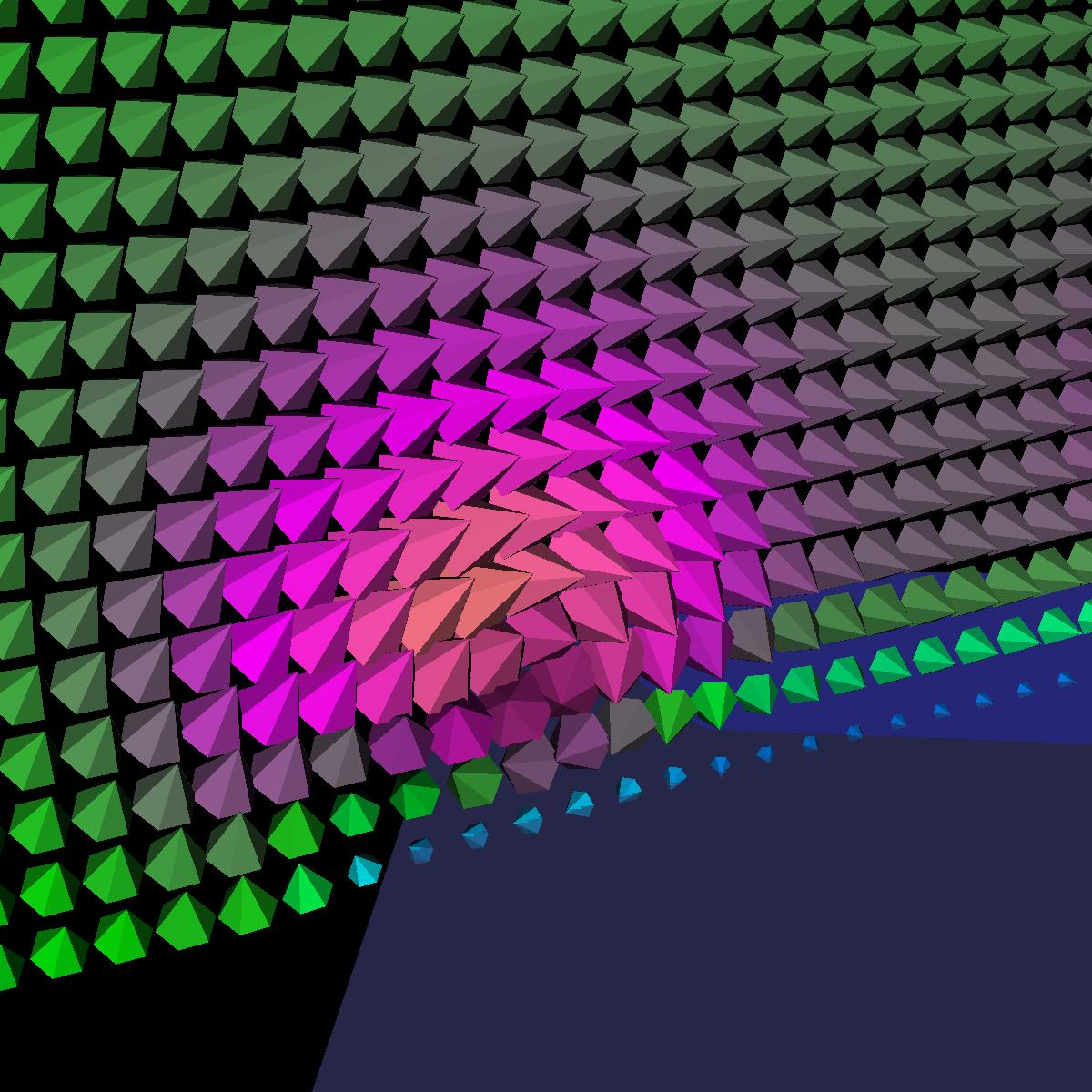 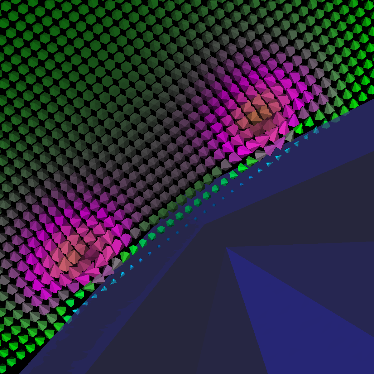 |
|
The four images below are rendered at location (70,0,0). 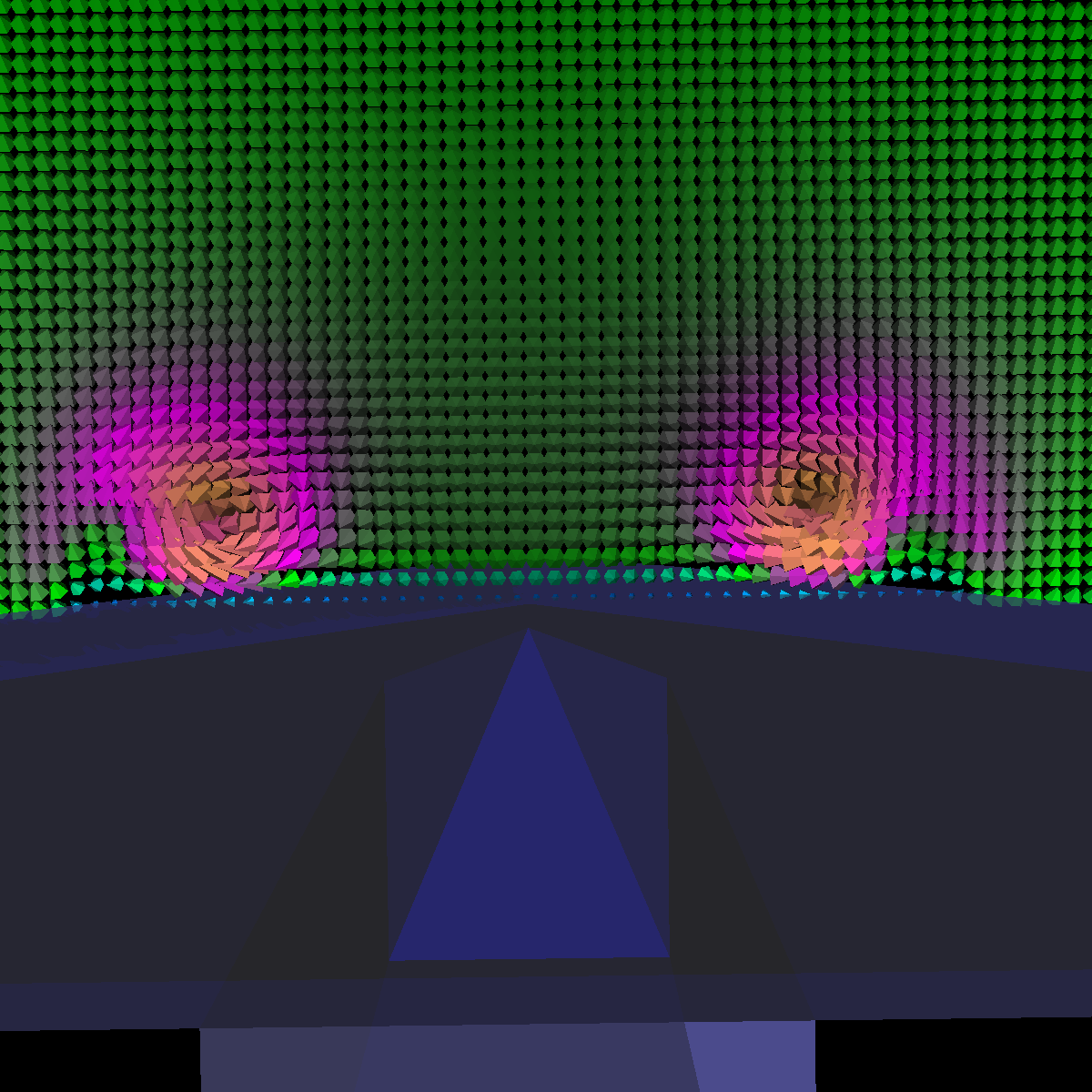 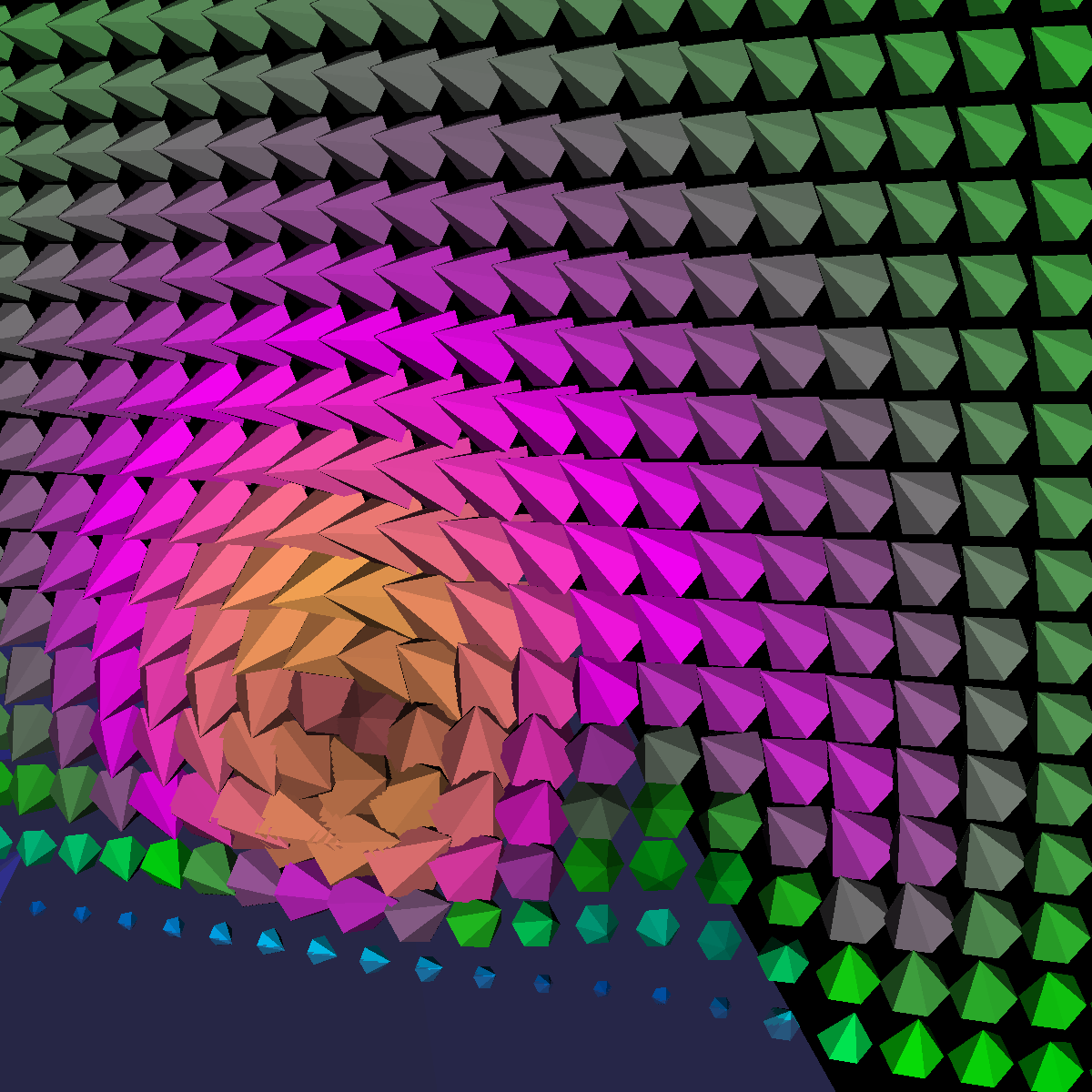 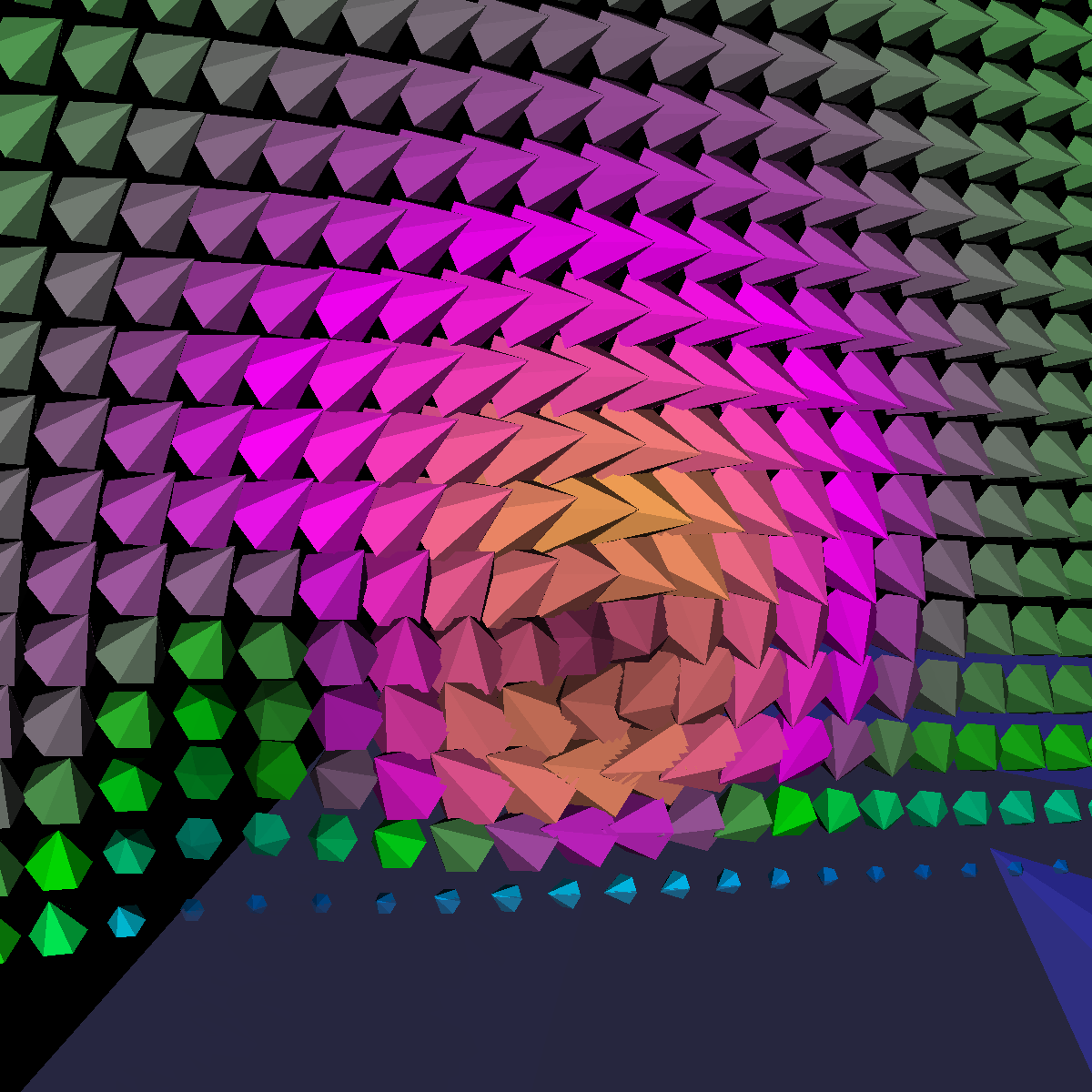 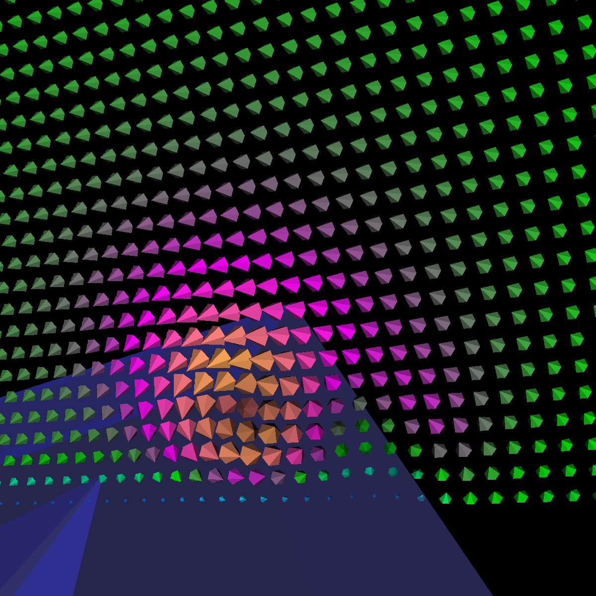 |
|
The four images below are rendered at location (150,0,0). 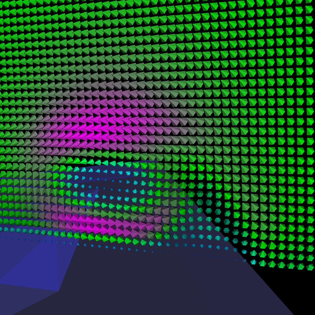 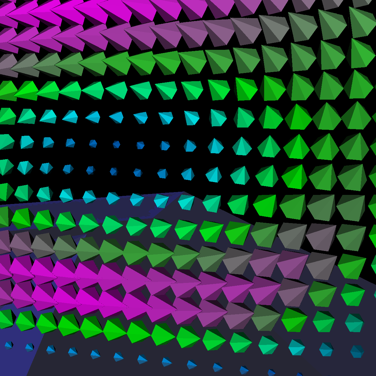 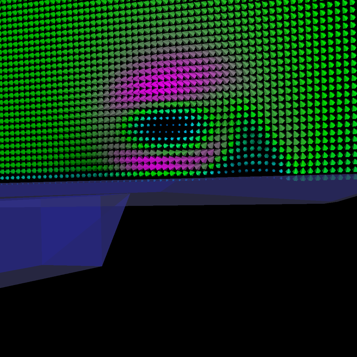 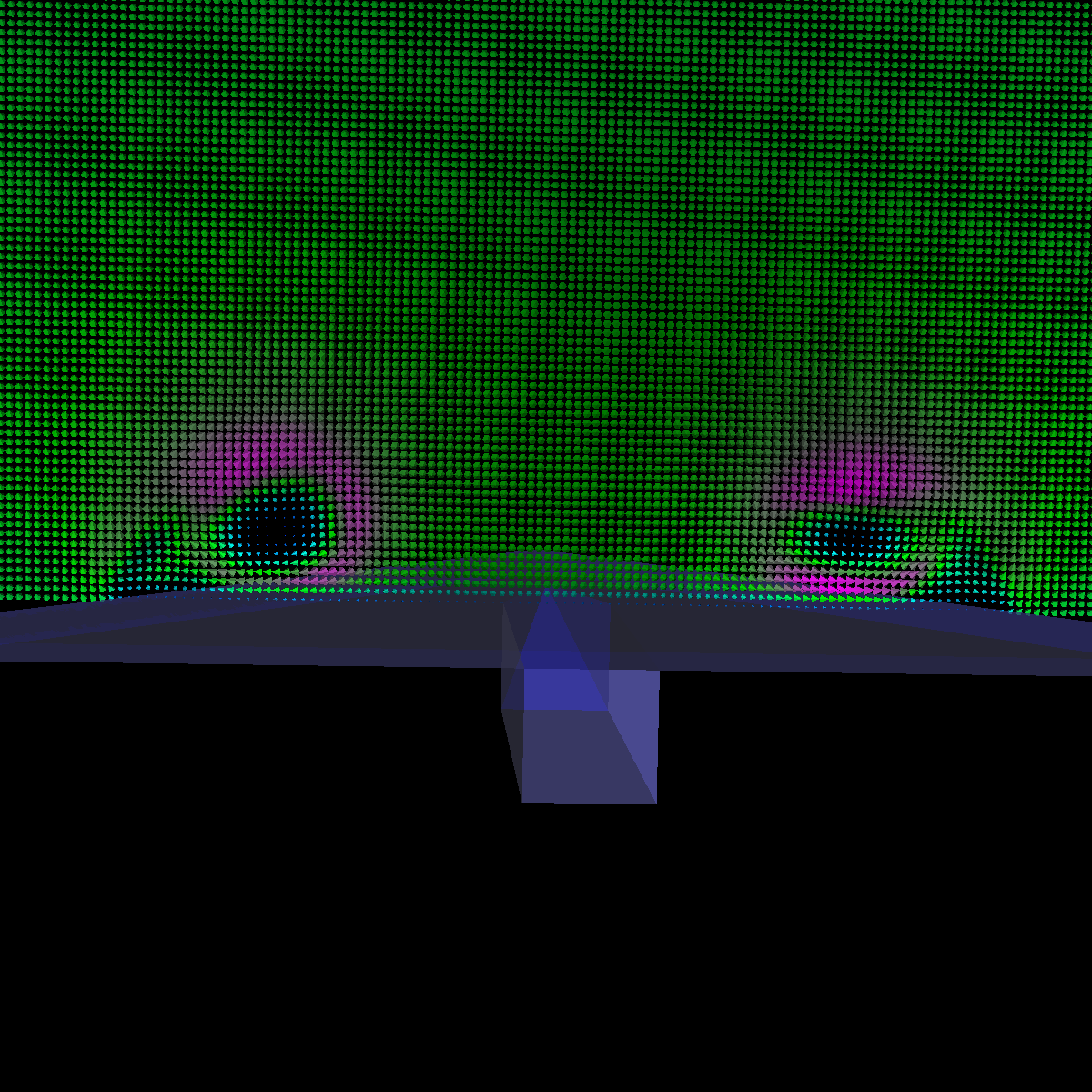 |
|
The two images below are rendered at location (110,0,0). 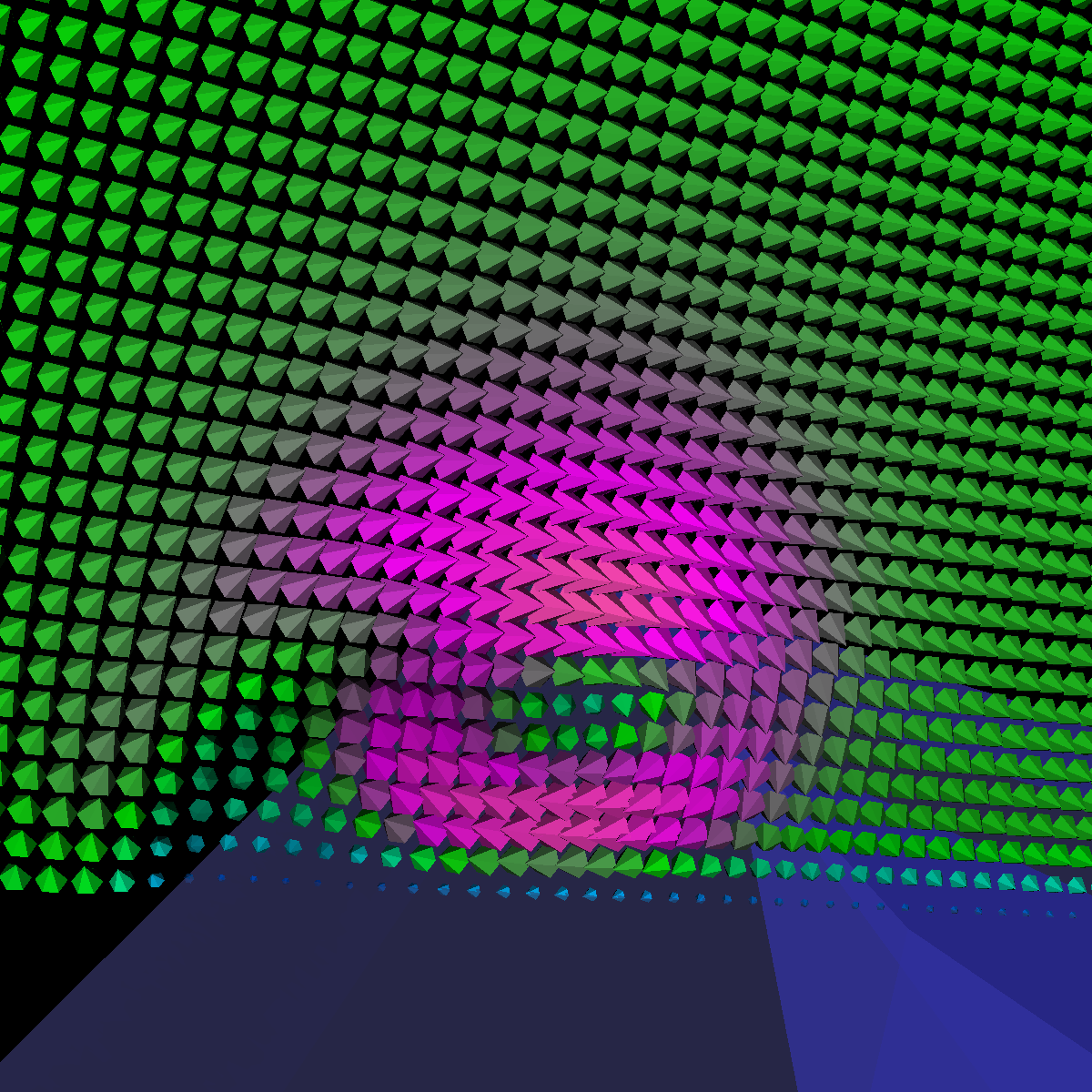 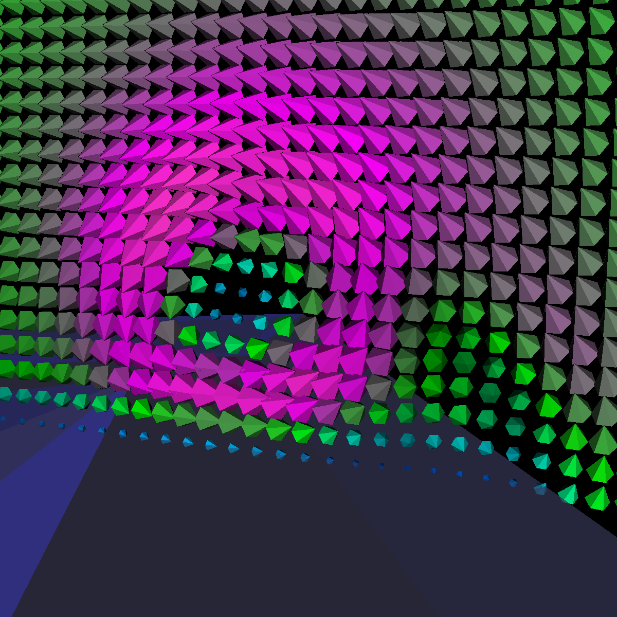 |
|
The four images below illustrate the plane at various other locations such as (25,0,0), (35,0,0), (130,0,0), and (170,0,0). 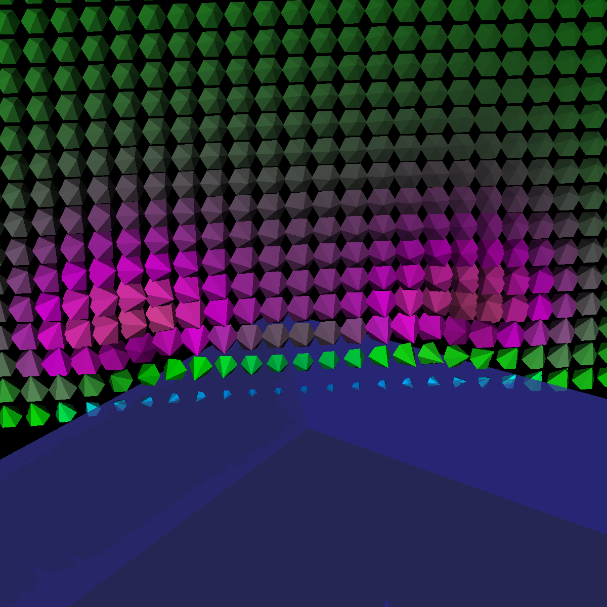 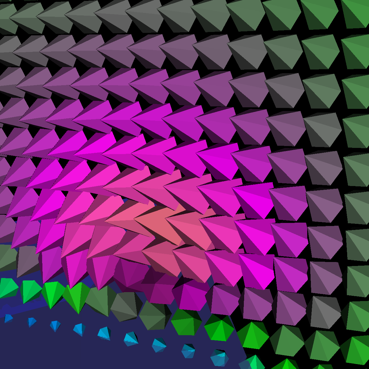 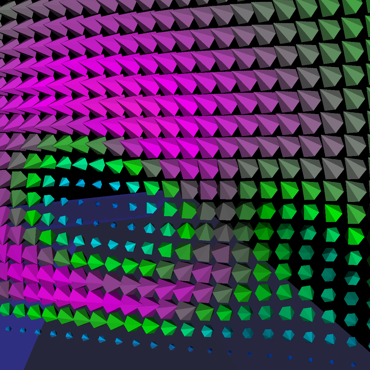 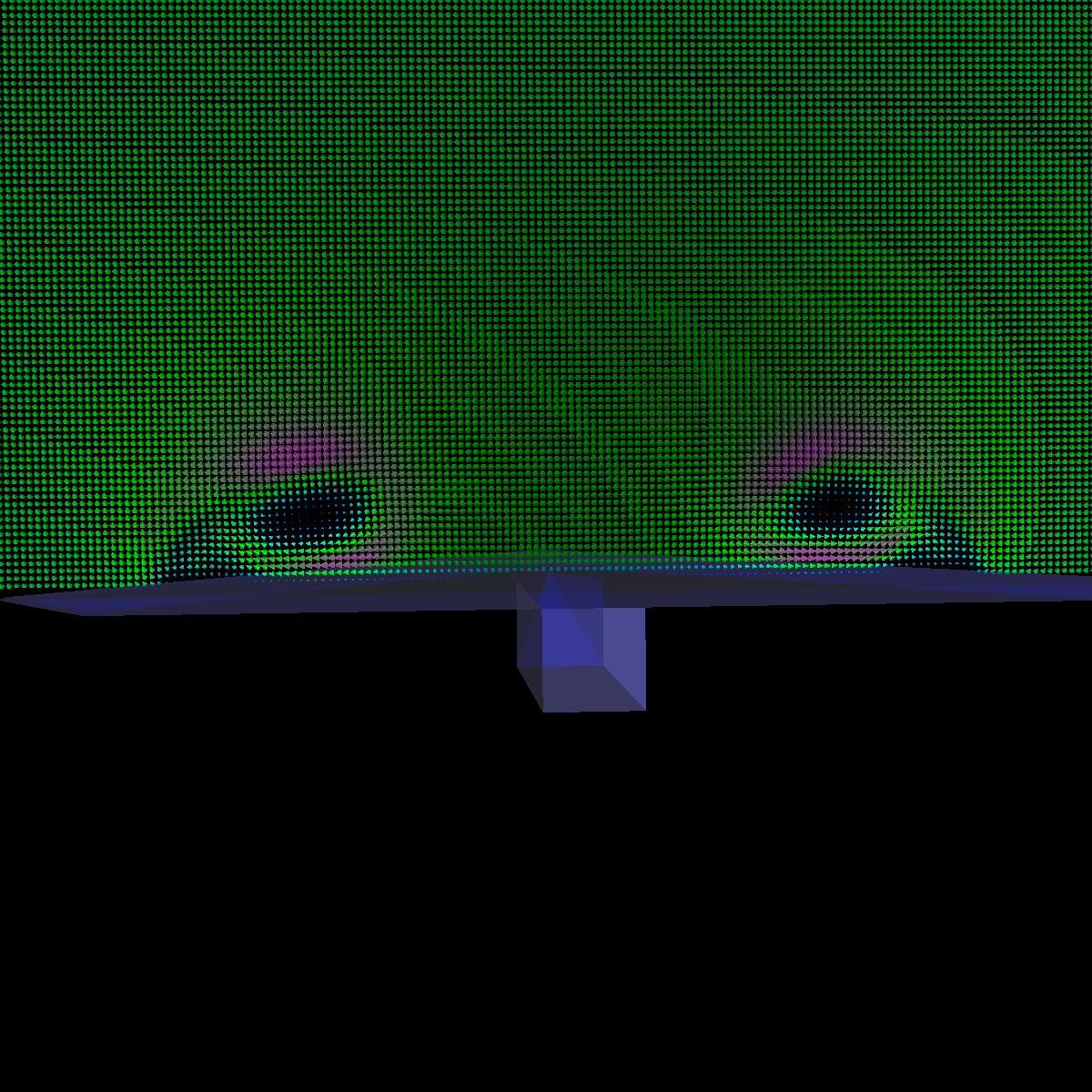 |
Part 1.2: Cylinder Glyphs |
|
The four images below are rendered at location (40,0,0). 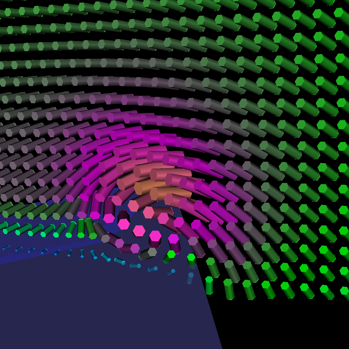 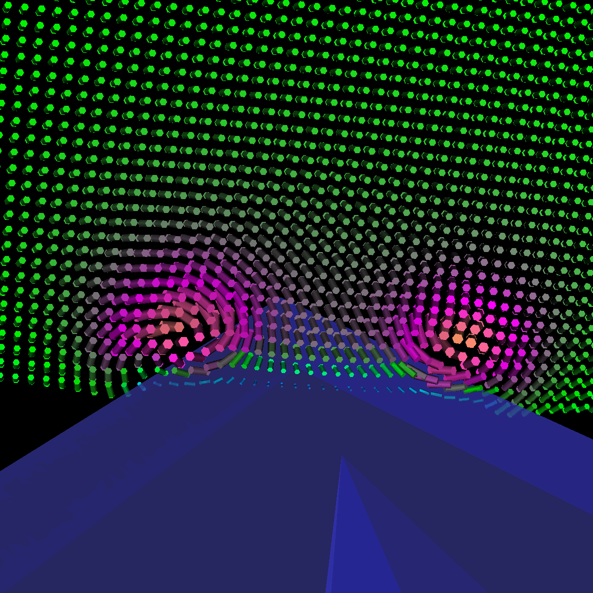 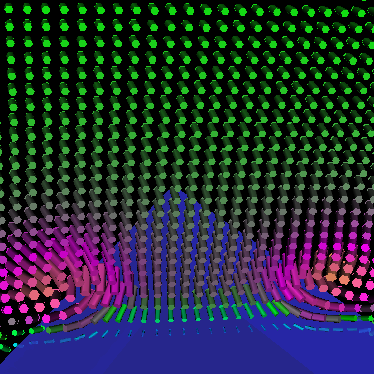 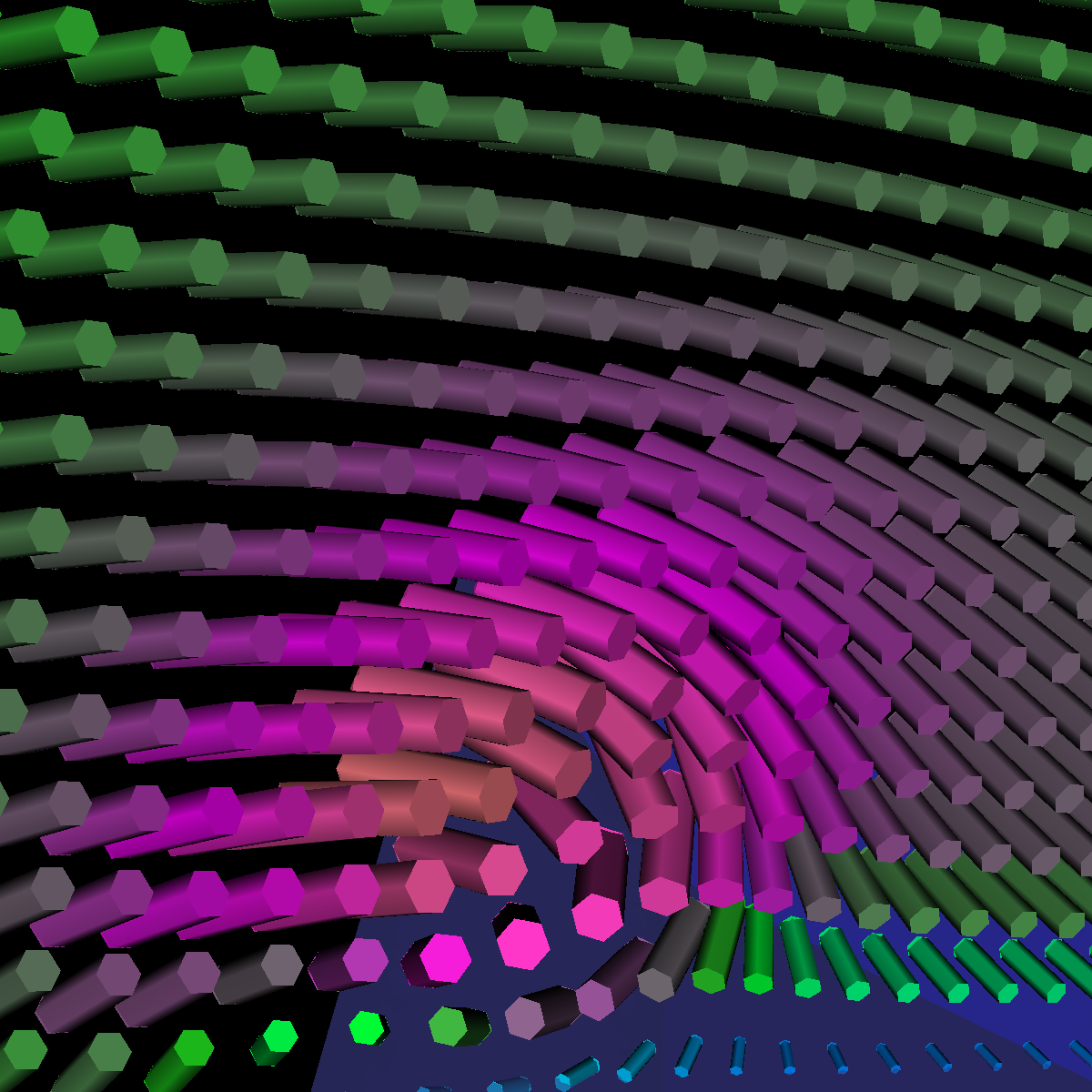 |
|
The four images below are rendered at location (70,0,0). 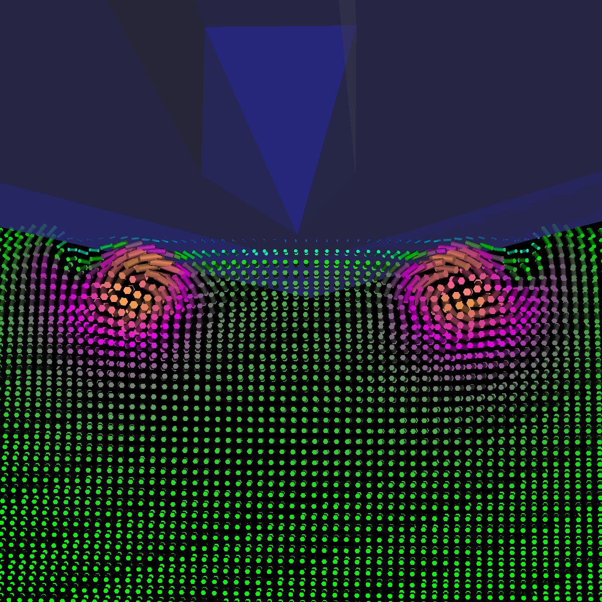 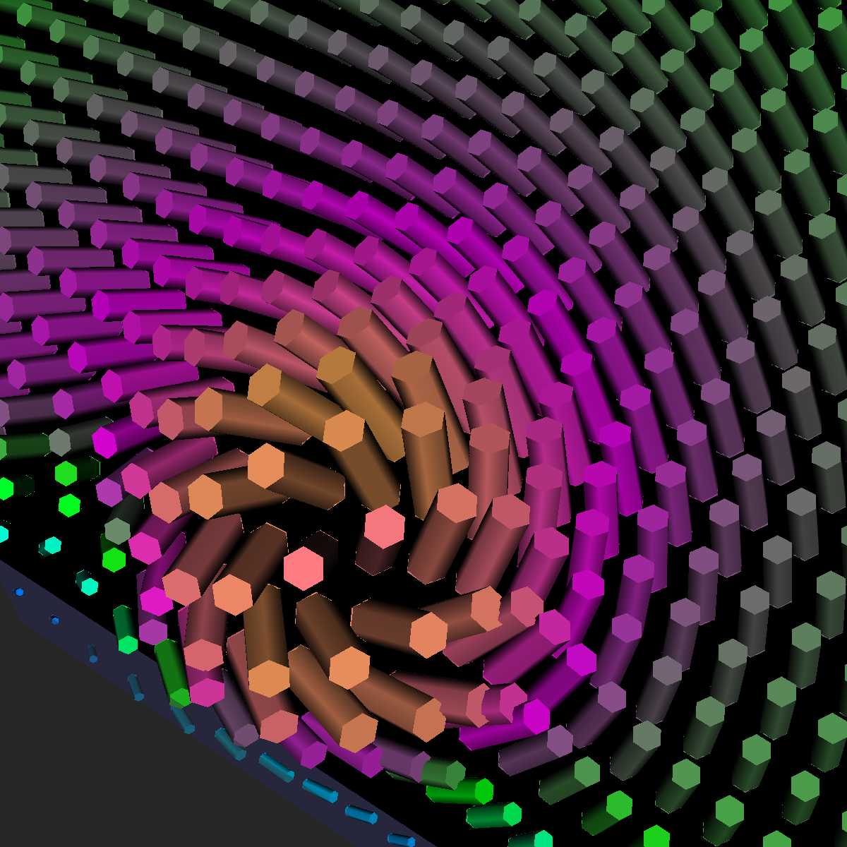  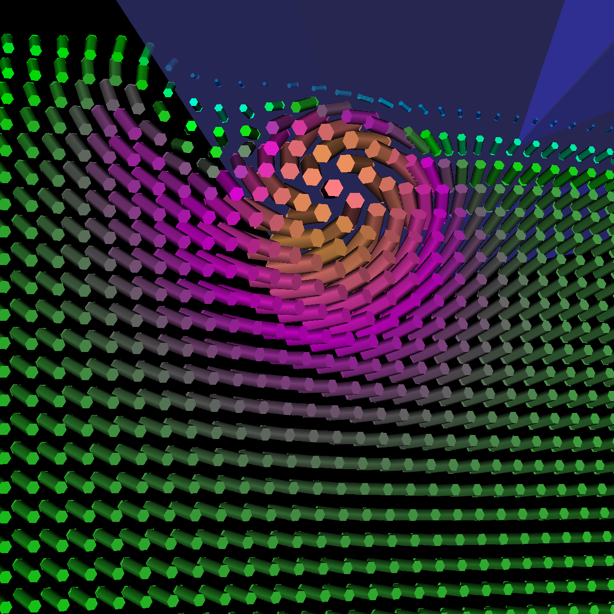 |
|
The four images below are rendered at location (150,0,0). 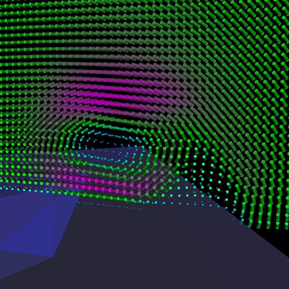  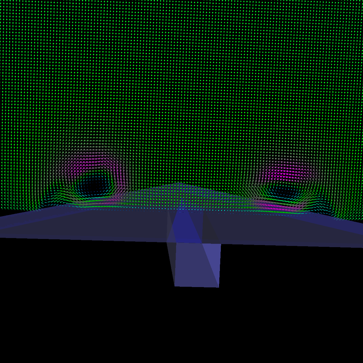 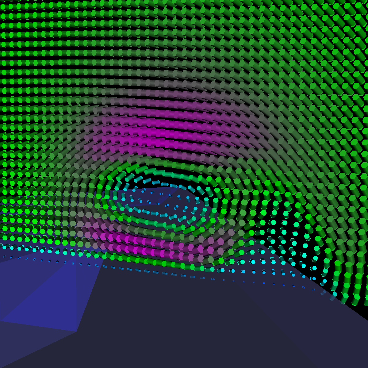 |
Part 1.3: Arrow Glyphs The two images below are rendered at location (40,0,0). 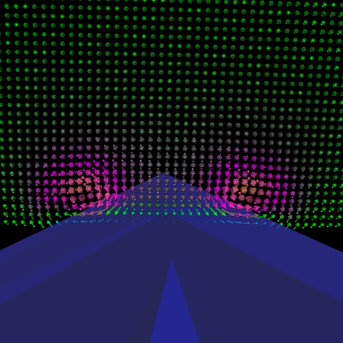 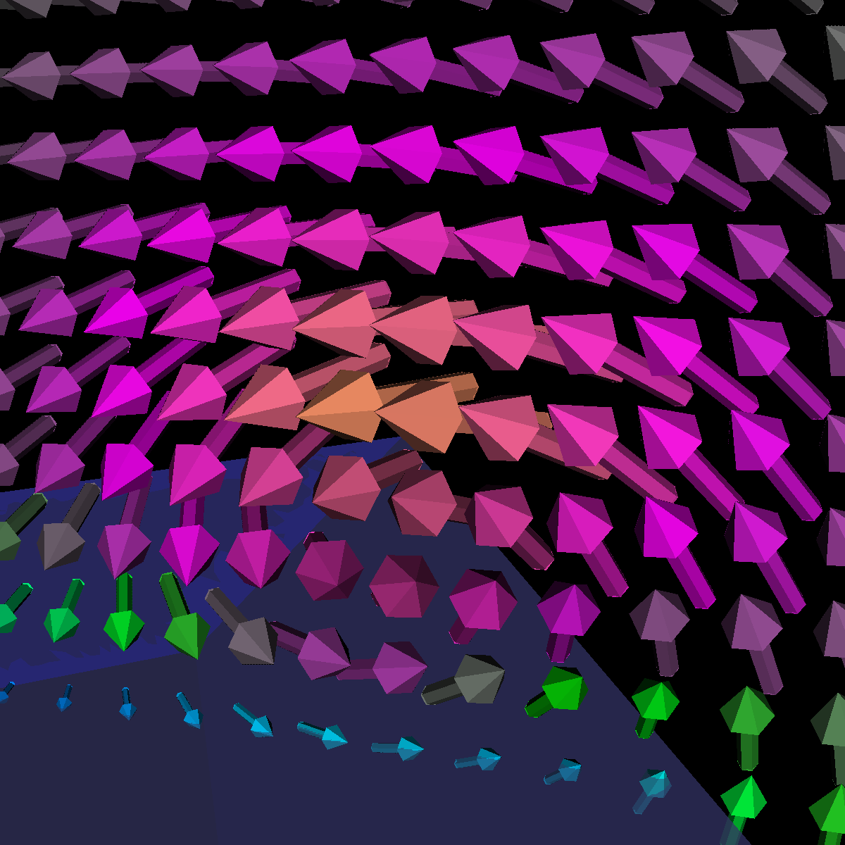 |
|
The two images below are rendered at location (70,0,0). 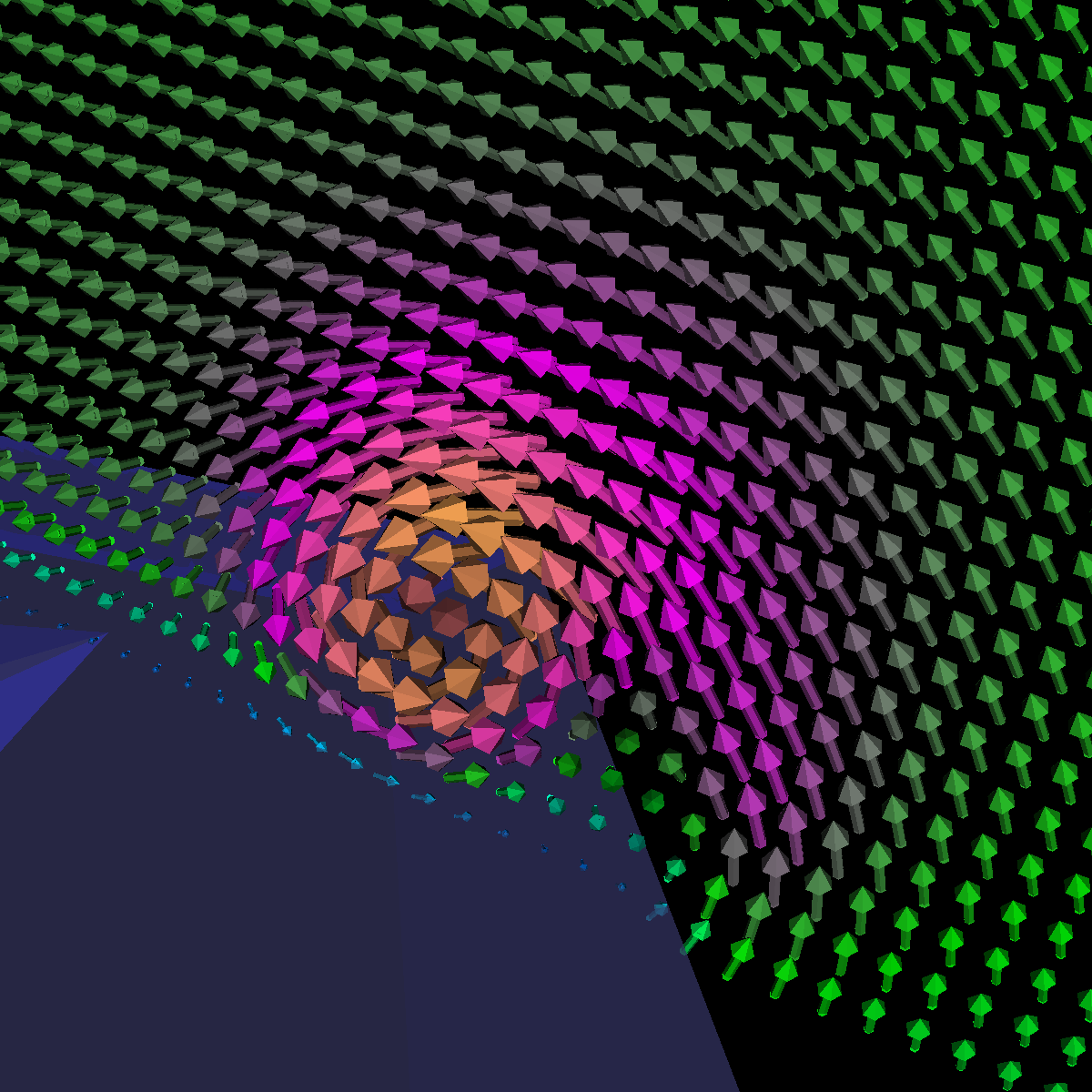 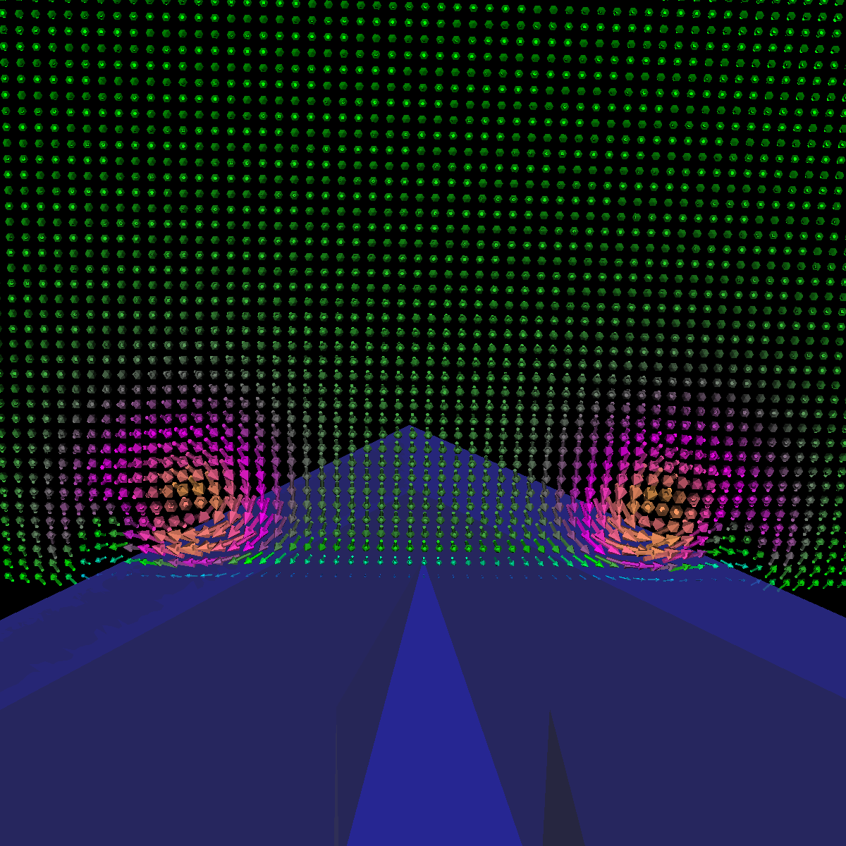 |
|
The two images below are rendered at location (150,0,0). 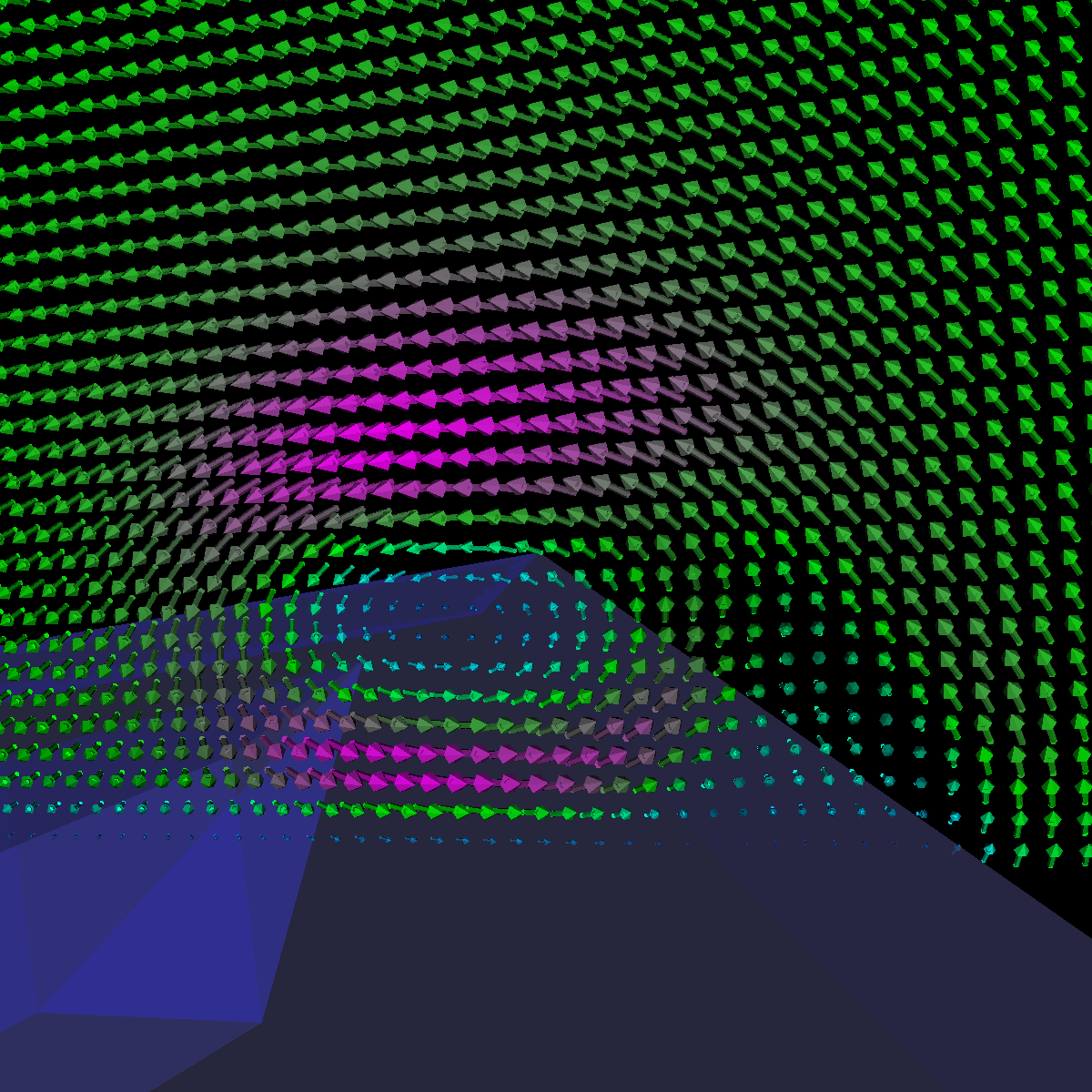 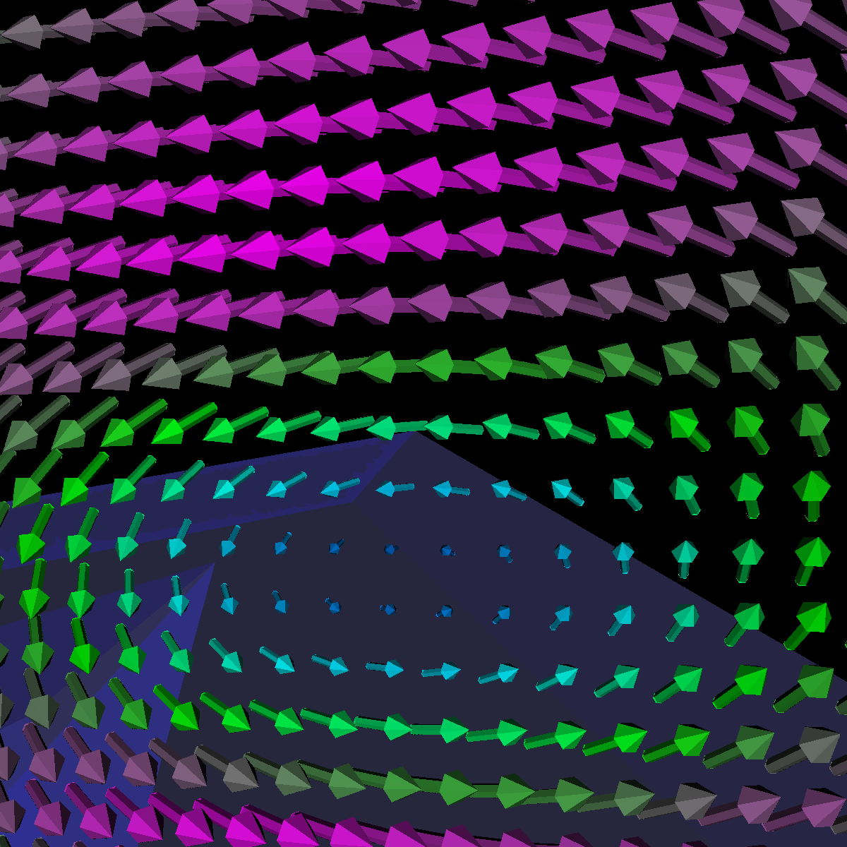 |
|
In the rendering below we positioned the plane in various locations. 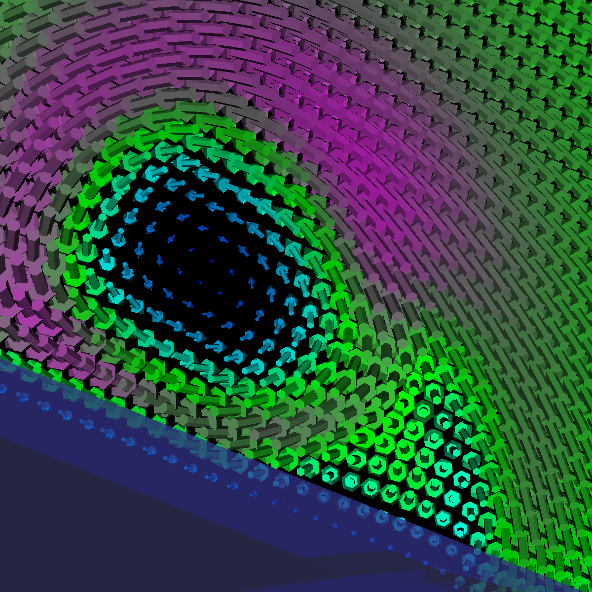 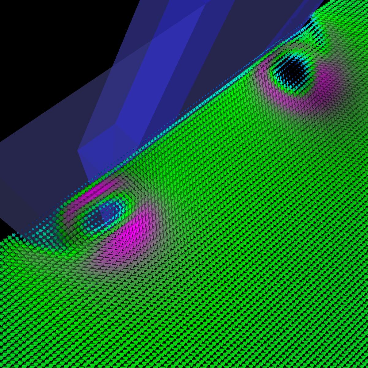 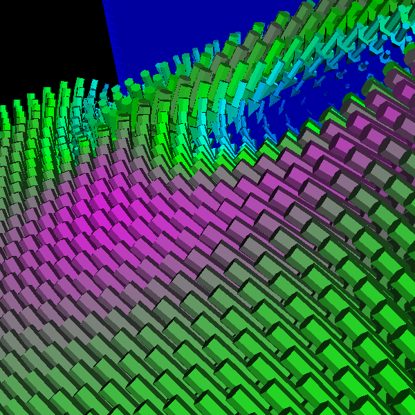 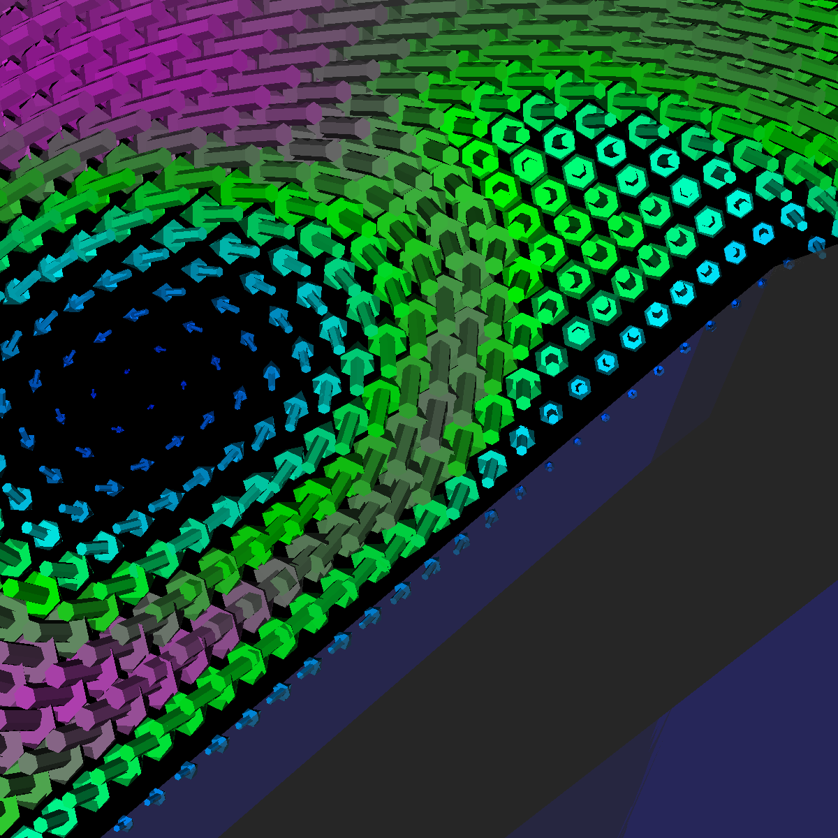 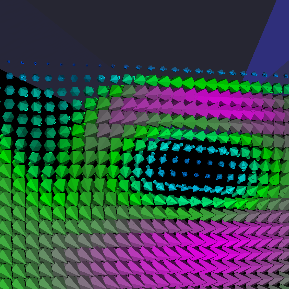 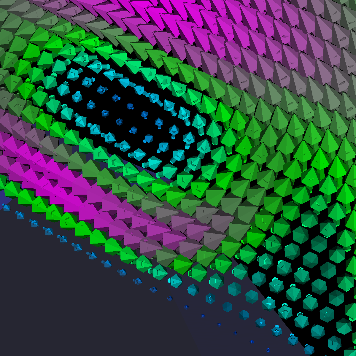 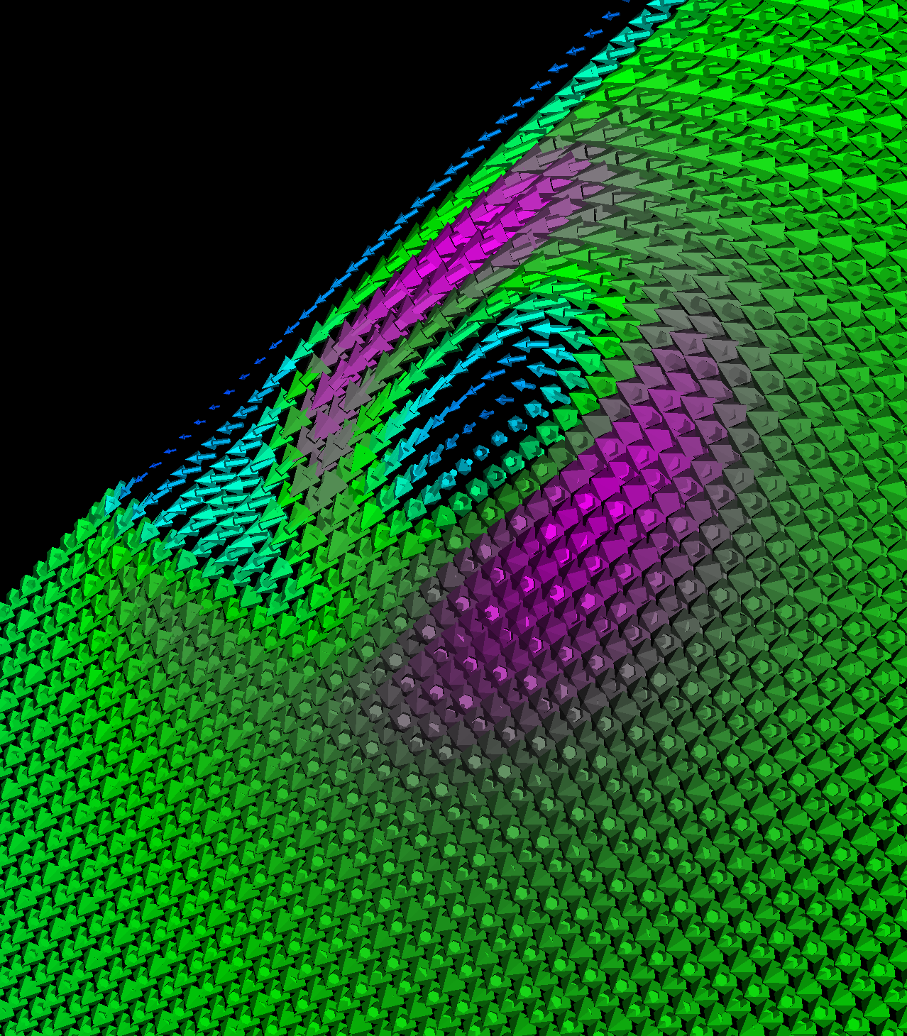 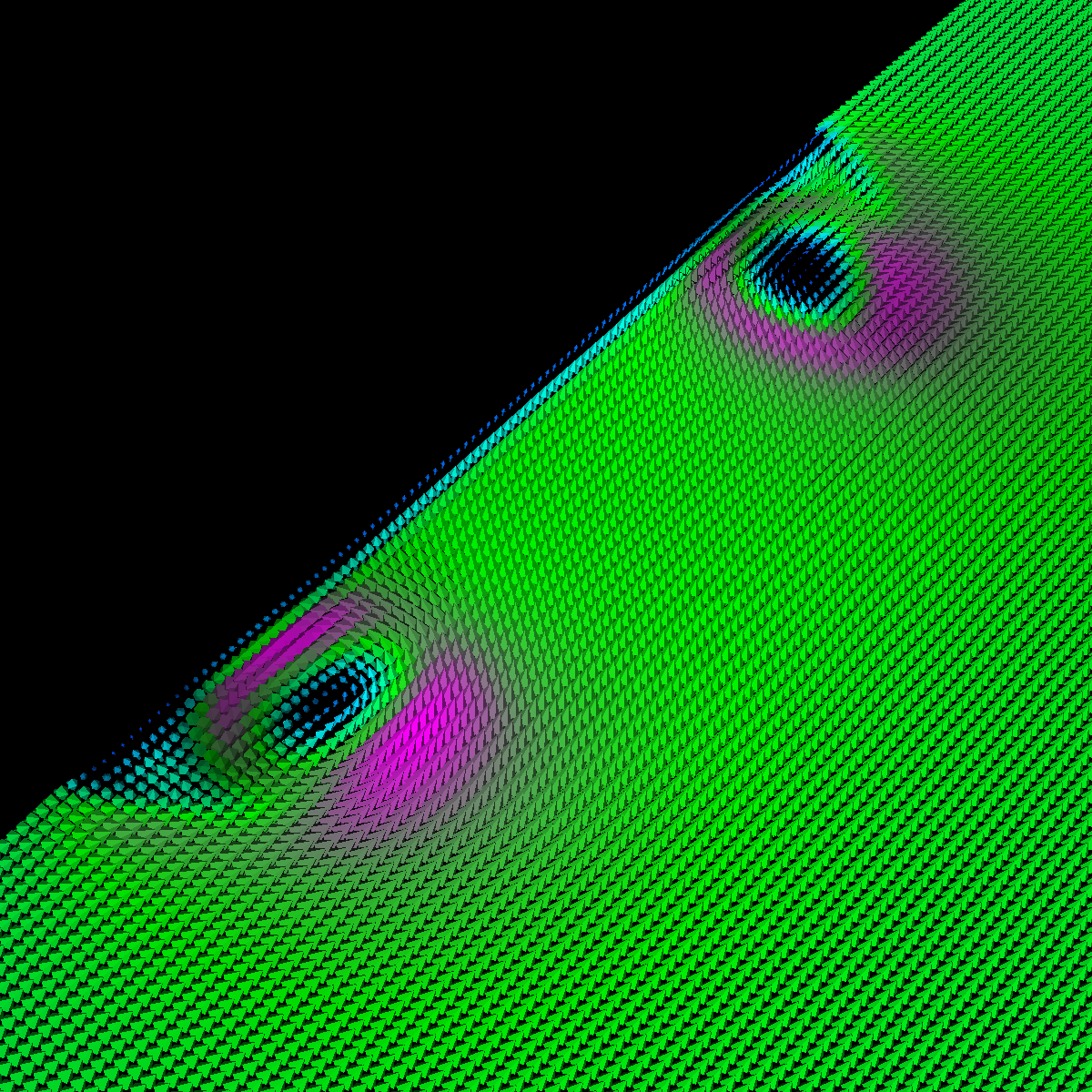 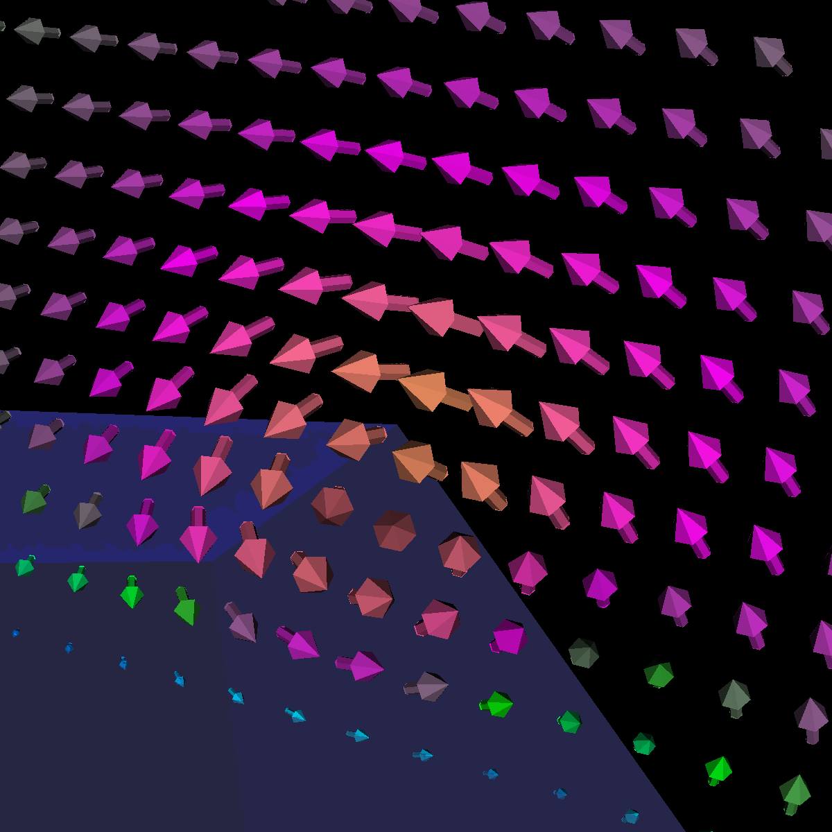 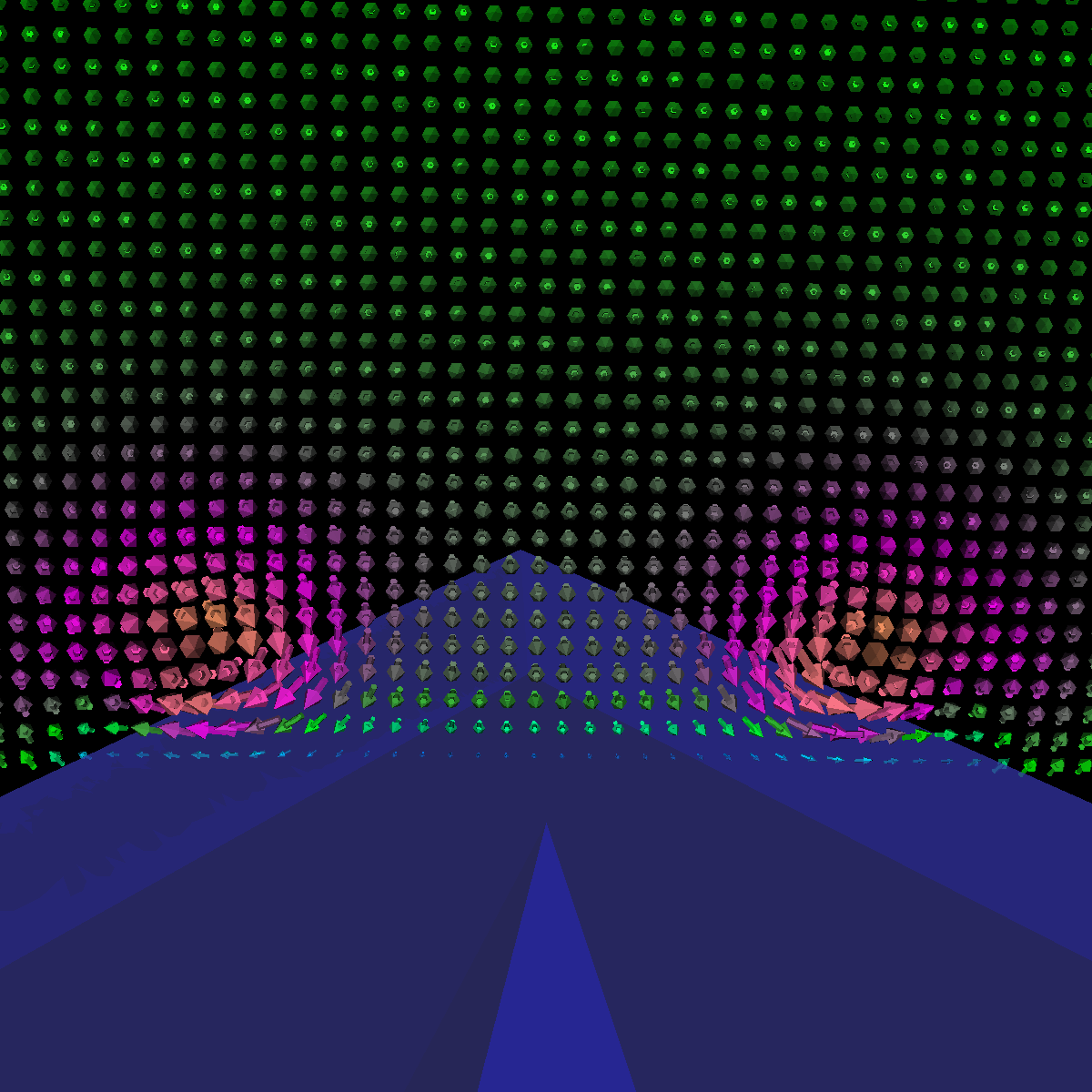 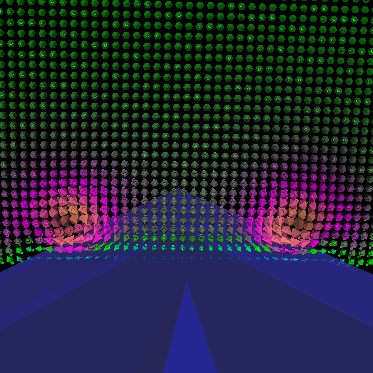 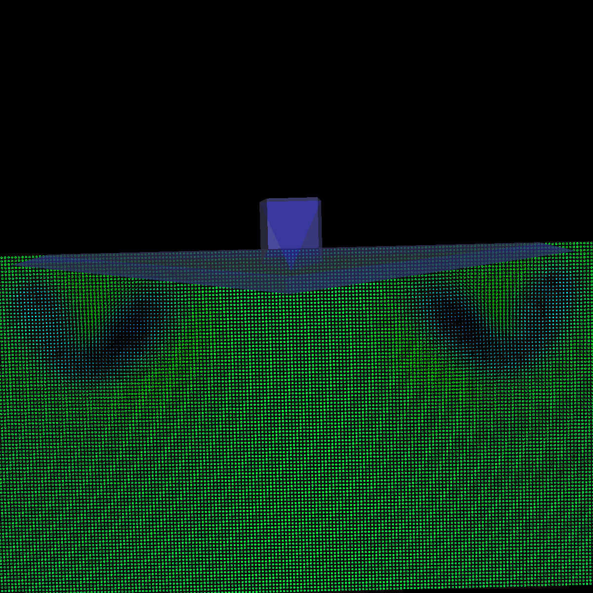 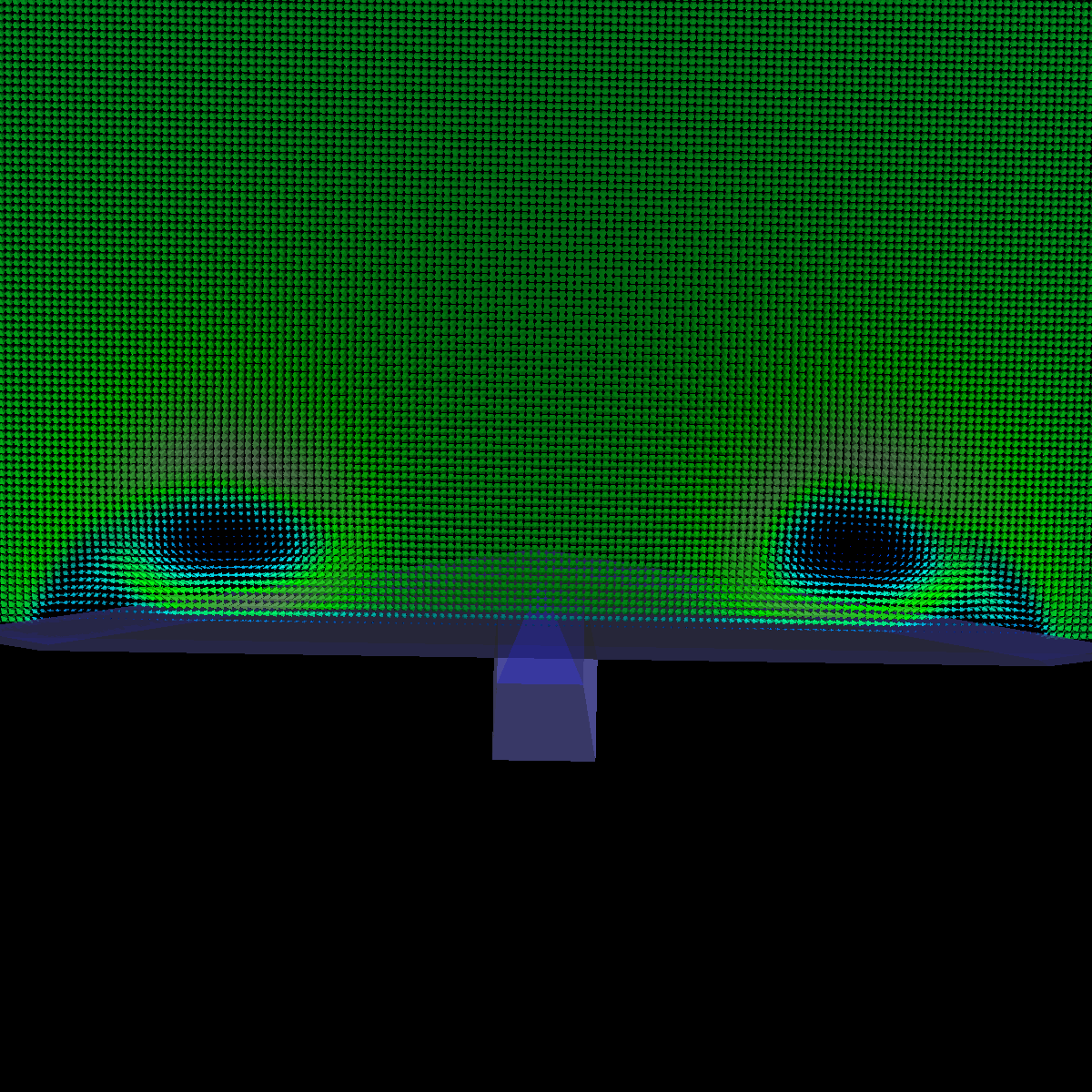 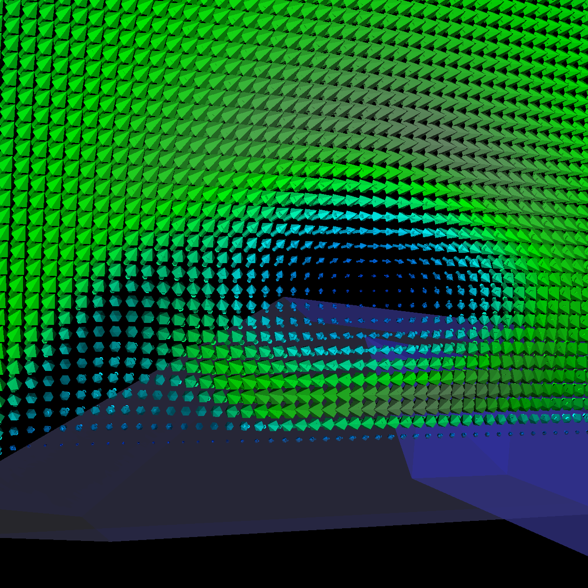 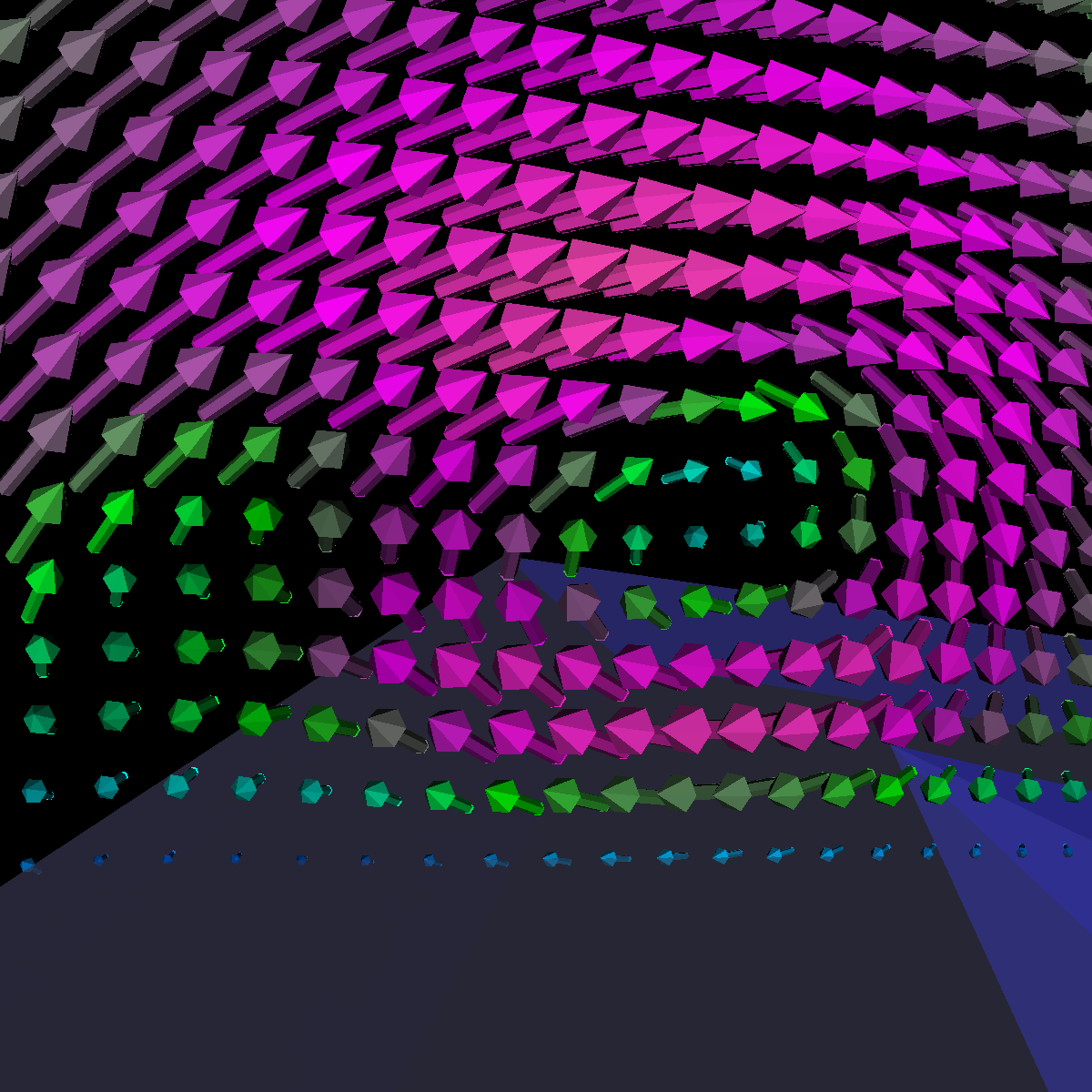 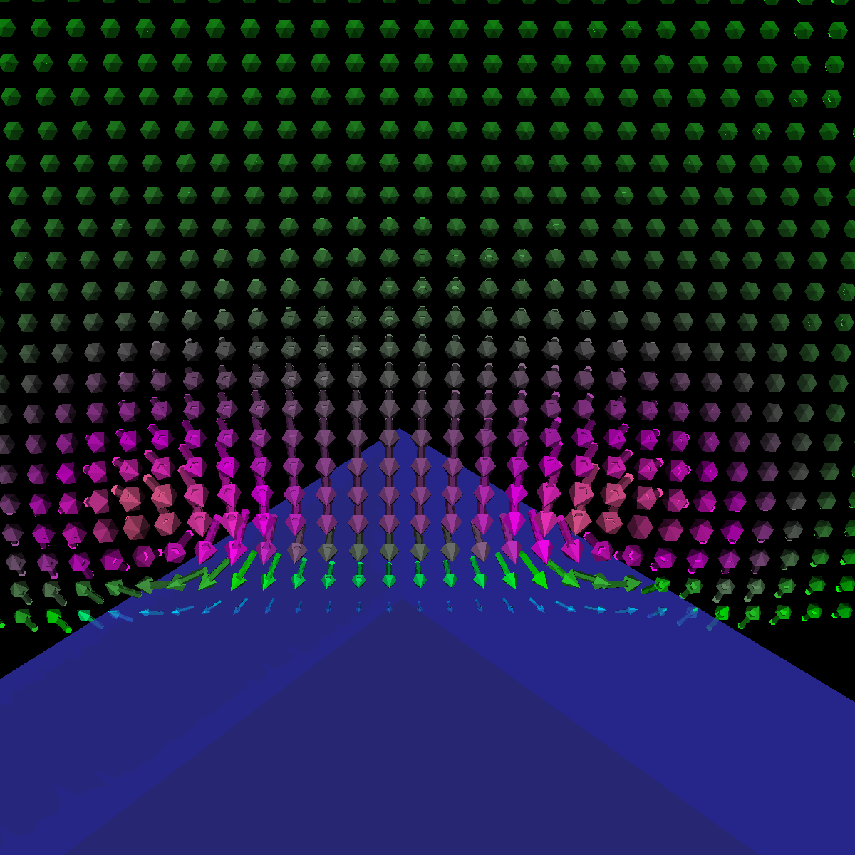 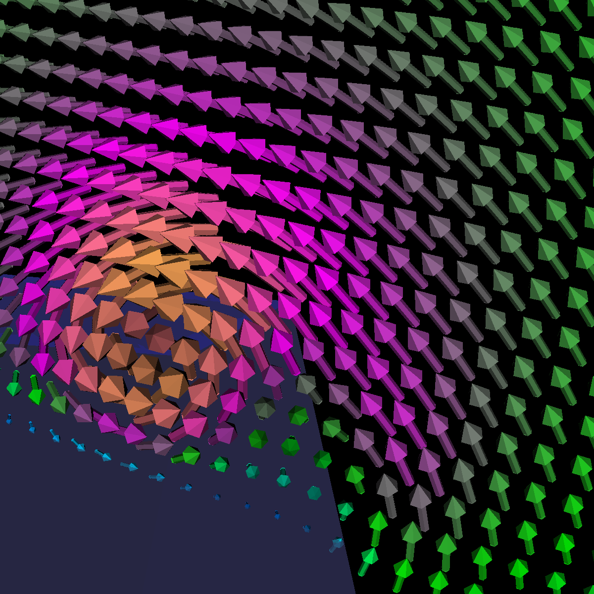 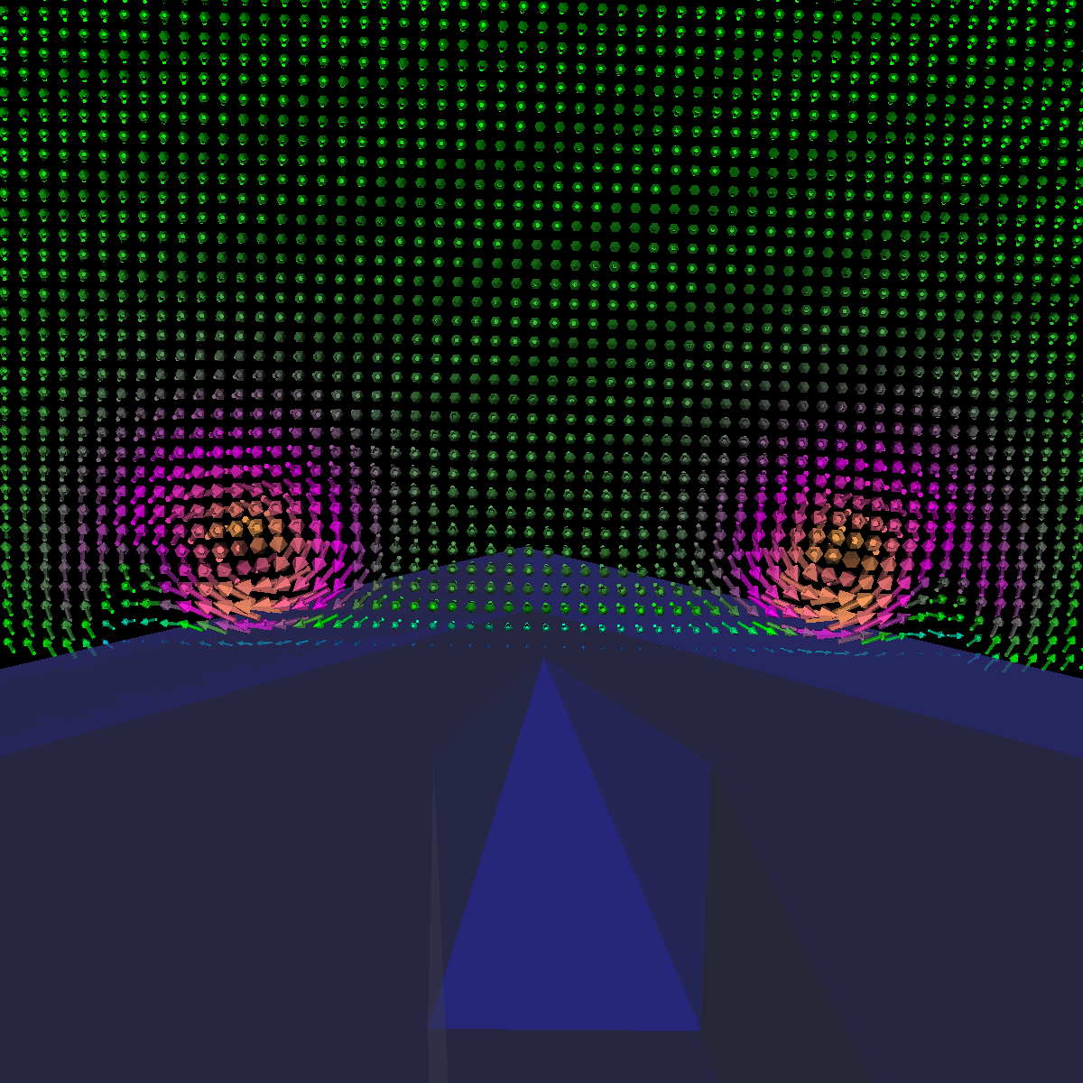 |
Part 1.4: Glyph Comparison: Cones, Cylinders, Arrows Question. How did we choose the plane locations and what observations led to that decision. The plane locations were chosen by first finding an appropriate view of the vortices and then sliding the plane along the x-axis and identifying interesting features in the process. We found locations such as (40,0,0) corresponds to the vortices formations as shown above. Furthermore, as we increasingly slide the plane, the spirals of the vortices also increases. The arrow glyphs are the most suitable as the direction and context is captured. The cones only show the direction whereas the cylinders sometimes fail to show the direction of the flow. However, the cylinders show the context as they bend with the flow whereas the cones fail to show the context. However, when combined to form arrows, then both the direction and context of the flow is captured. We provide a detailed comparison below and discuss further the utility of the sampled plane locations. |
Part 1.4.1: Glyph Comparision: (40,0,0) Sampled Plane Position We chose to sample the velocity field at location (40,0,0). This sampled plane position provides insight into the formation of the first vortices. In the visualizations below (from left-to-right: arrow, cones, cylinders), we appropriately capture the formations using arrows and cylinders. The cylinders provide a unique effect as we clearly see them bend around one another with the flow whereas this effect is slightly less pronounce using arrows. The cones in this case only provides the direction of the flow. |
Part 1.4.2: Glyph Comparision: (70,0,0) Sampled Plane Position This sampled plane position captures the other vortice which is beginning to form. We also see the progression of the center vortice. The arrows provide a more intuitive representation of the flow as it circulates around the first vortice and from the secondary vortices. |
Part 1.4.3: Glyph Comparision: (150,0,0) Sampled Plane Position The sampled plane position is located toward the back of the wings and provides a more global view as the remaining vortices are shown. This visualization shows the velocity magnitude in the center vortice decreases significantly while the velocity magnitude of the particles further from the center vortices increases. We also see that the velocity magnitude is greatest on either side of the center vortice and decreases as it flows in between. Furthermore, the other vortices flow directions are also captured. As before, the arrows clearly provide the most intuitive representation of the flow. |
|
|
Part 2: Streamlines, Stream Tubes, and Stream Surfaces We use streamlines, stream tubes, and stream surfaces to capture the flow around the vortices on each side of the wing. The velocity magnitude of the rendered primitives is color coded. Question. How are the seeding locations chosen and how do they relate to the observations made using glyphs with cutting planes? We chose the seeding locations from using the information discovered by visualizing the vector field using glyphs where we slide a cutting plane across the x-axis. From this technique we observe where each of the primary, secondary and tertiary vortices initially arise and use this intuition for seeding. We also selected some seeding locations to capture other interesting features (i.e., recirculation bubble). We initially used four primary seeding locations. The first set is centered at (40,20,0) for the vortices along the left wing and the other center is at (40,-20,0) capturing the right wing vortices. Further, at these two seeding locations we used a radius of 12 and seeded 30 points. These two points capture the significant vortices. To capture other interesting features, we also created two more seeding locations centered at (70,50,0) for the left wing and (70,-50,0) for the right wing. These locations have a raidus of 13 and consist of 40 points each. These seeding locations were again selected using the above procedure. We also tried various other seeding locations by slightly modifying the given locations. These locations are used for streamlines, stream tubes and stream ribbons. For stream surfaces we selected seeding locations along a generated line. Similar intuitions as previously discussed were used for selecting the initial location of the line (i.e., the two end points). |
Part 2.1: Streamlines 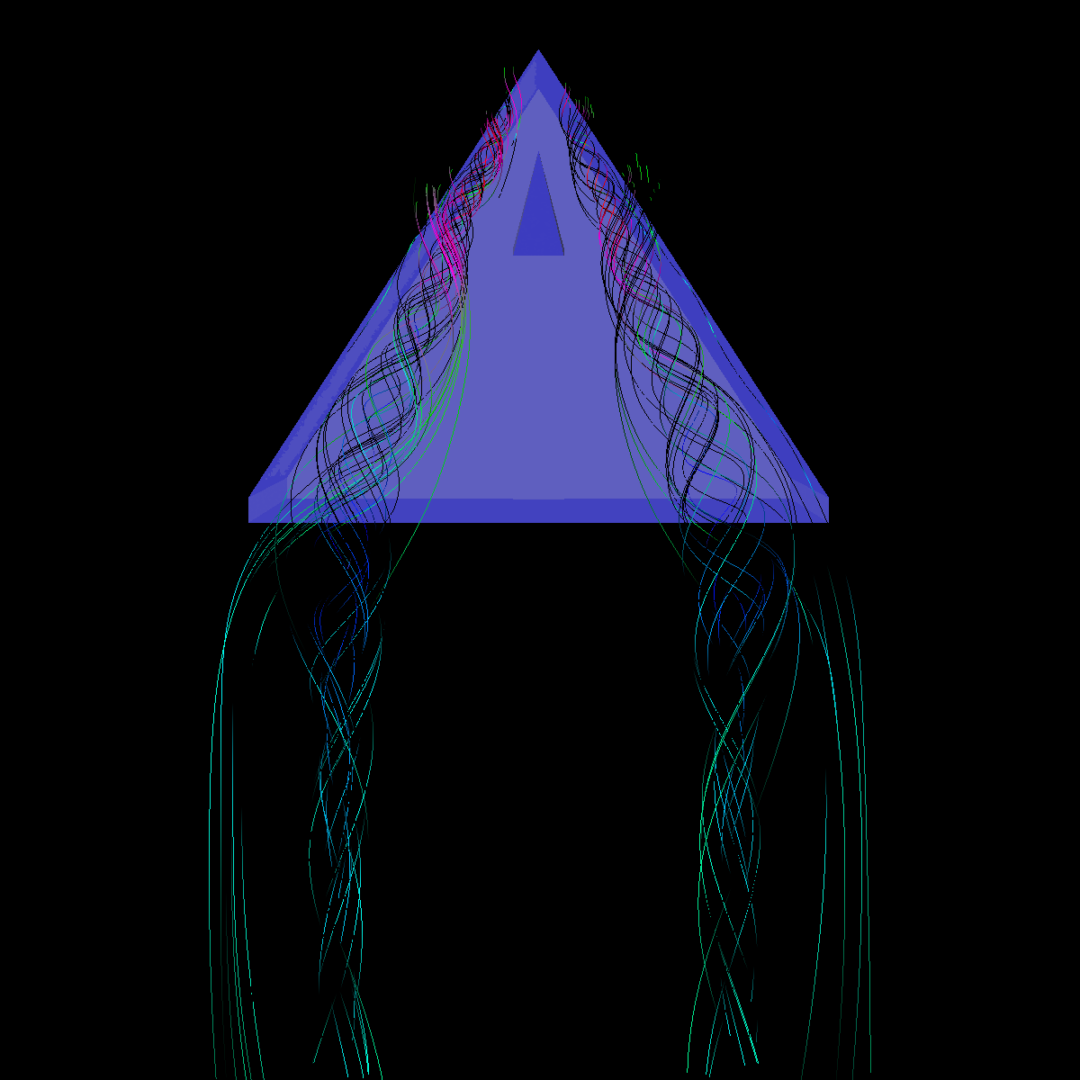 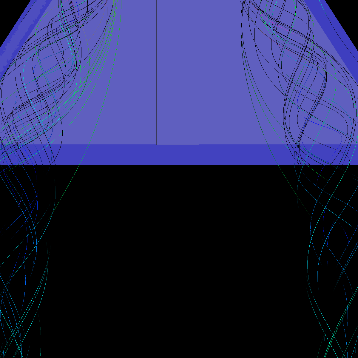 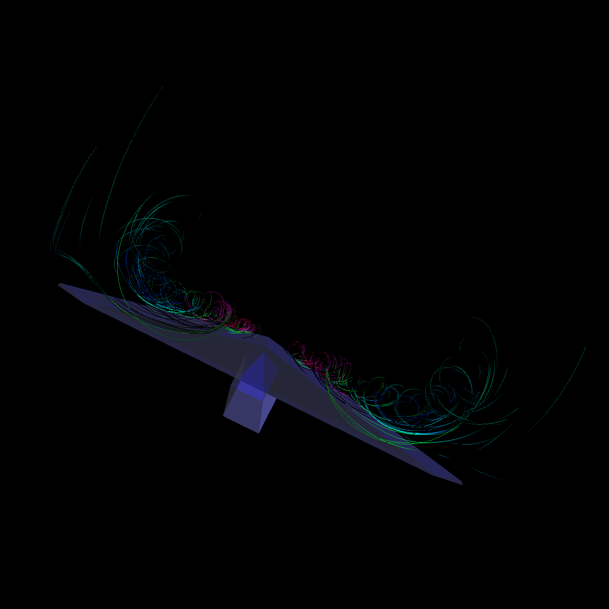 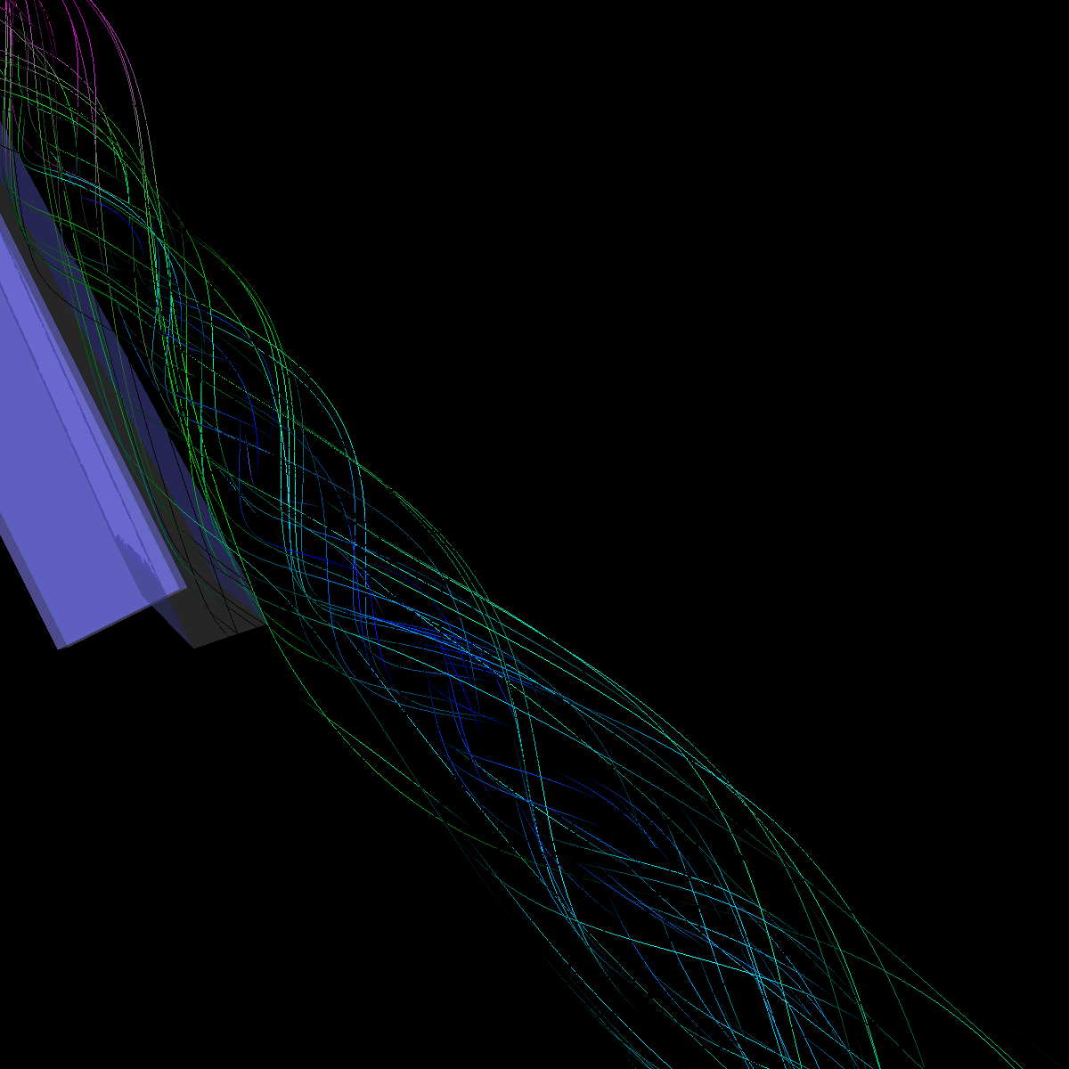 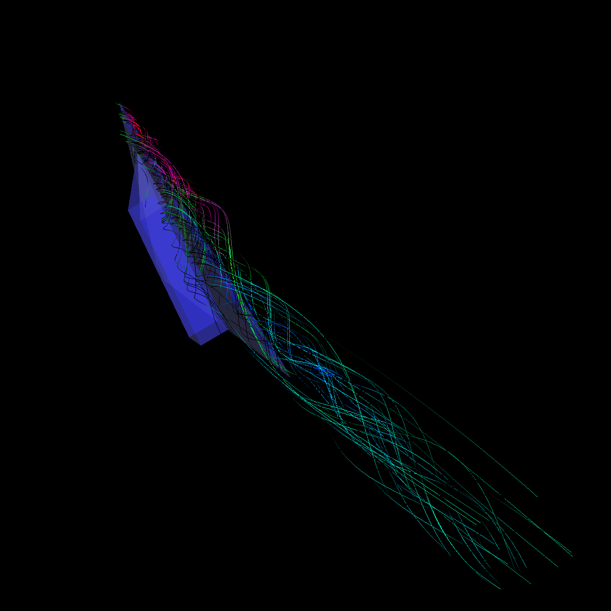 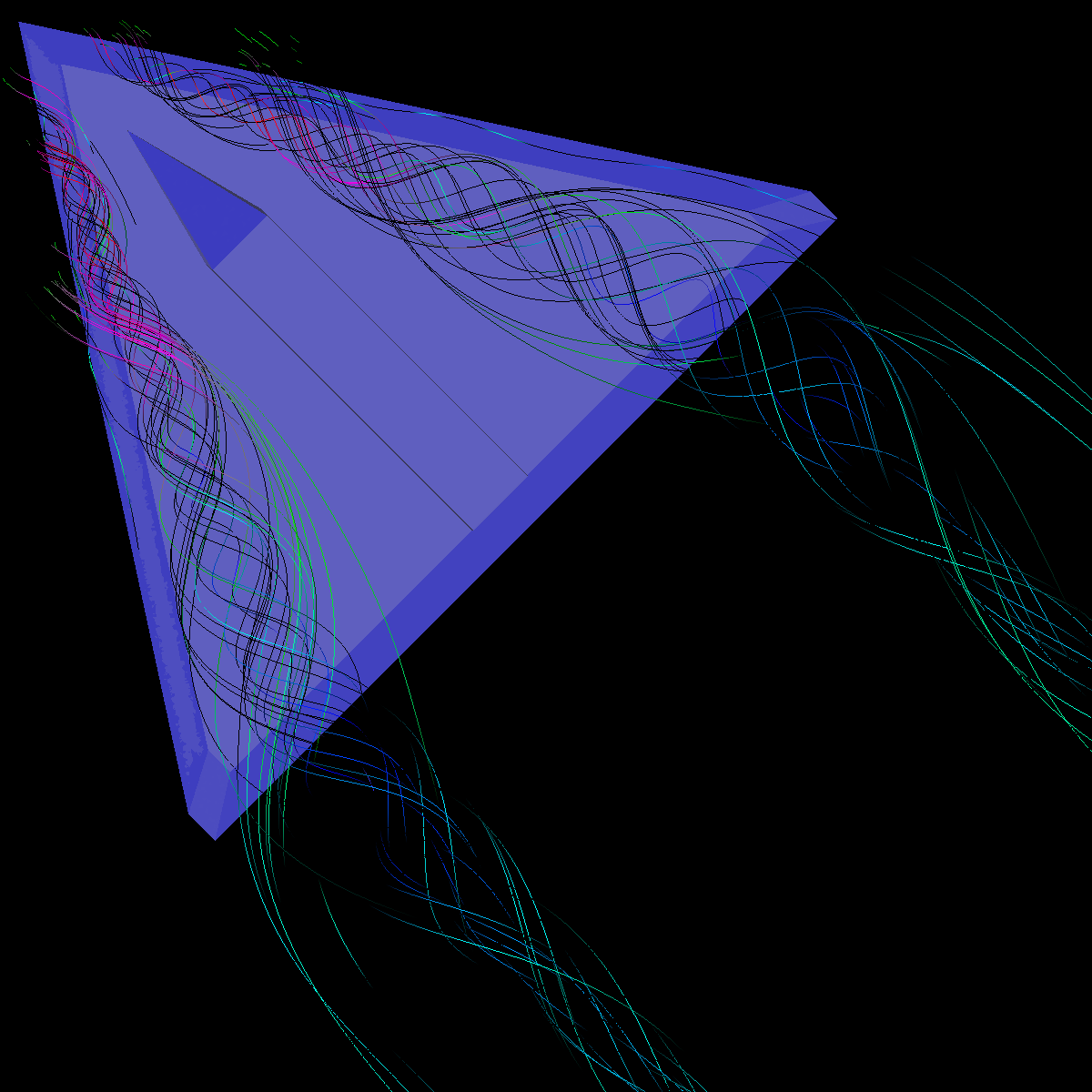 |
Part 2.1.1: Other Streamline Visualizations 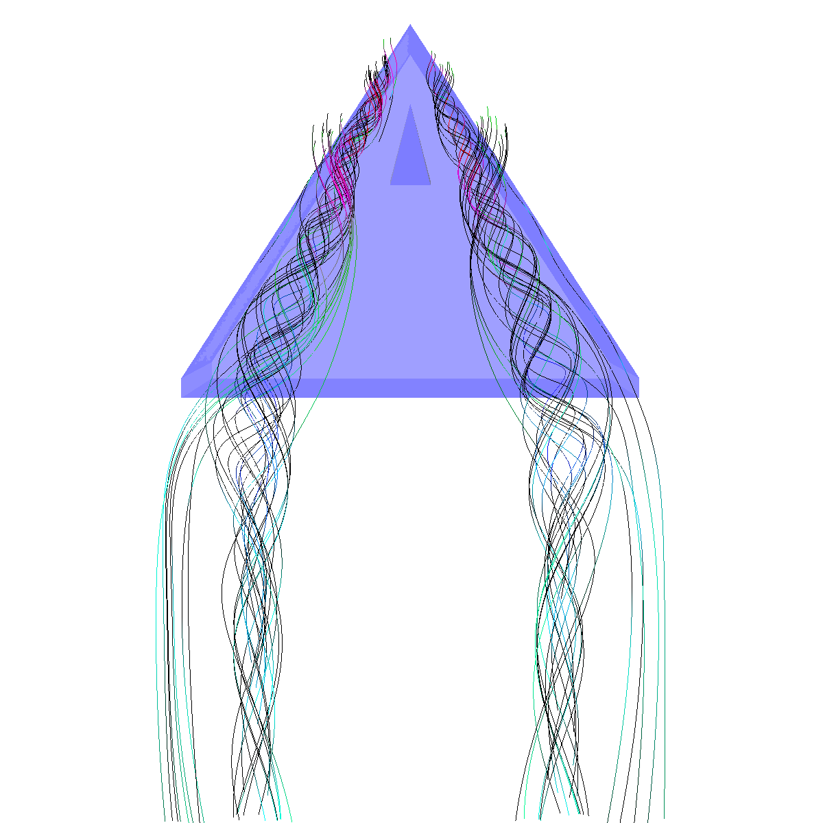 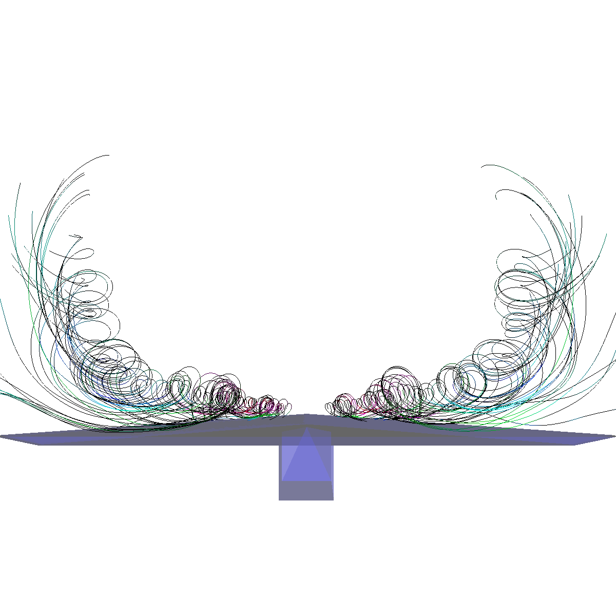 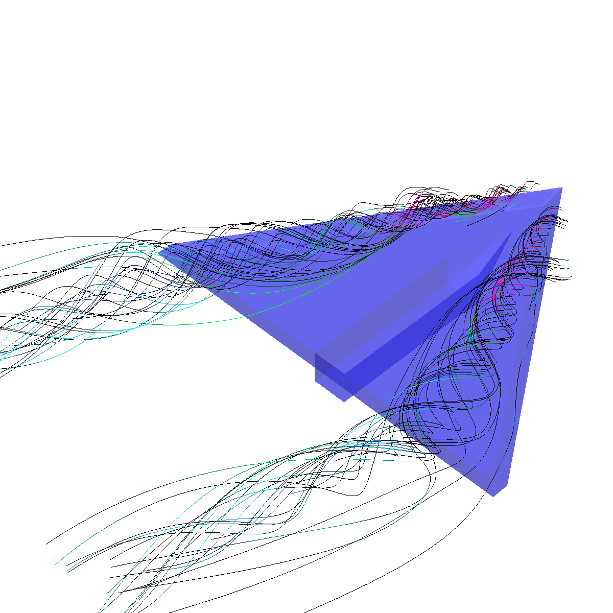 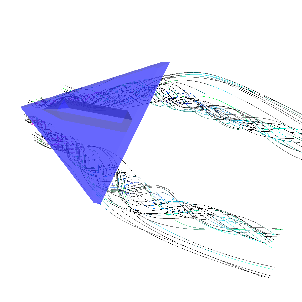 |
Part 2.2: Stream Tubes The stream tubes are much better than simply using streamlines as the width of each can change with respect to the velocity magnitude. 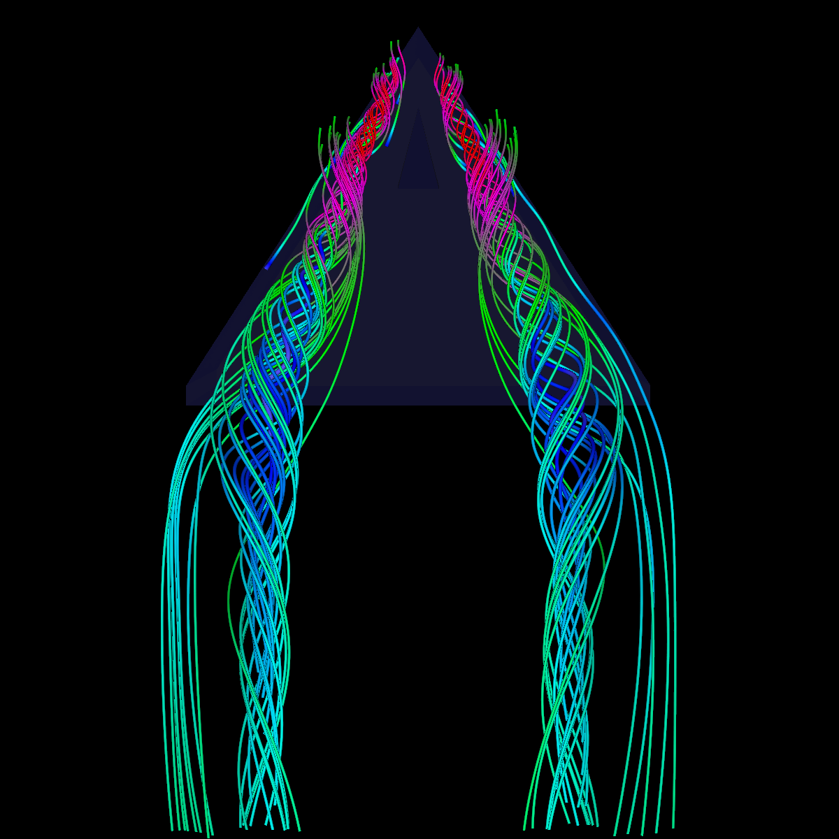 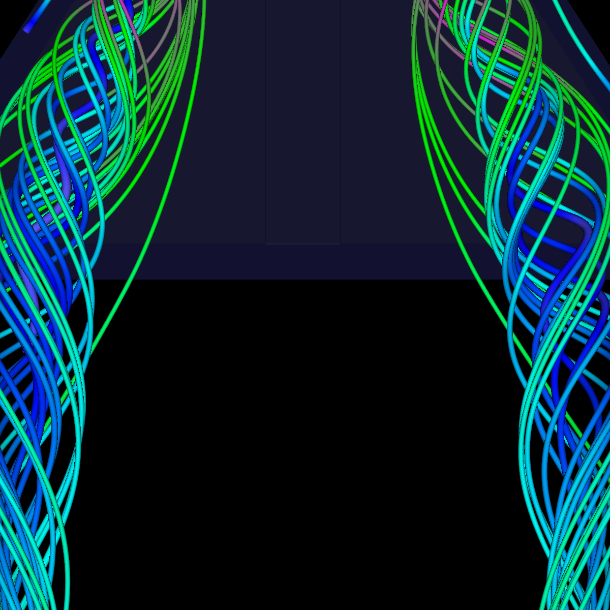 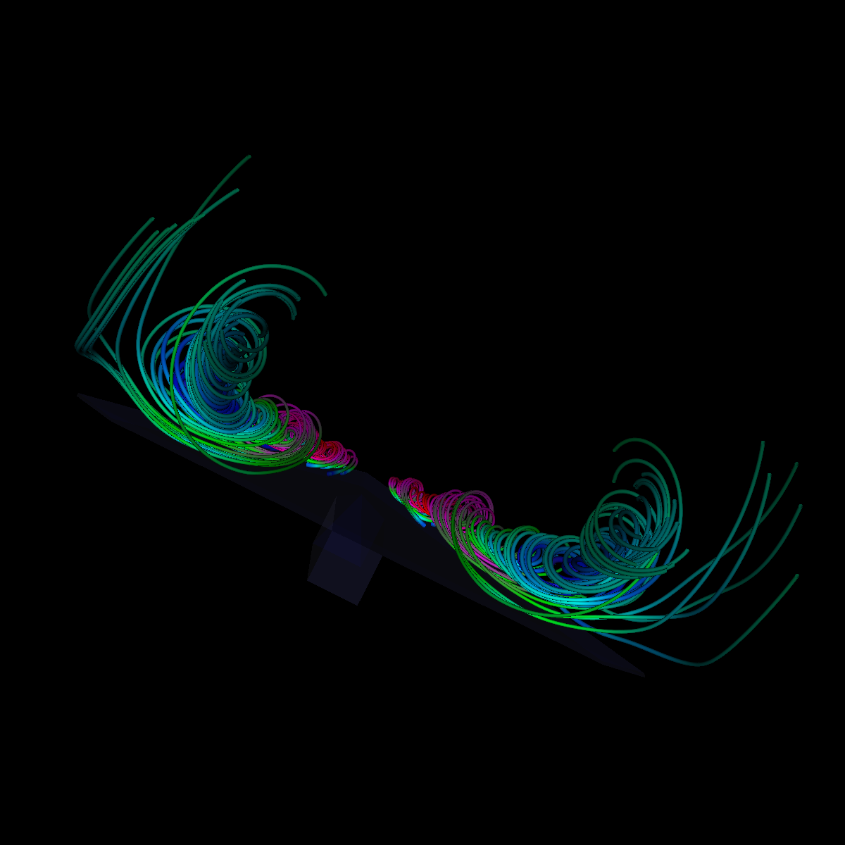 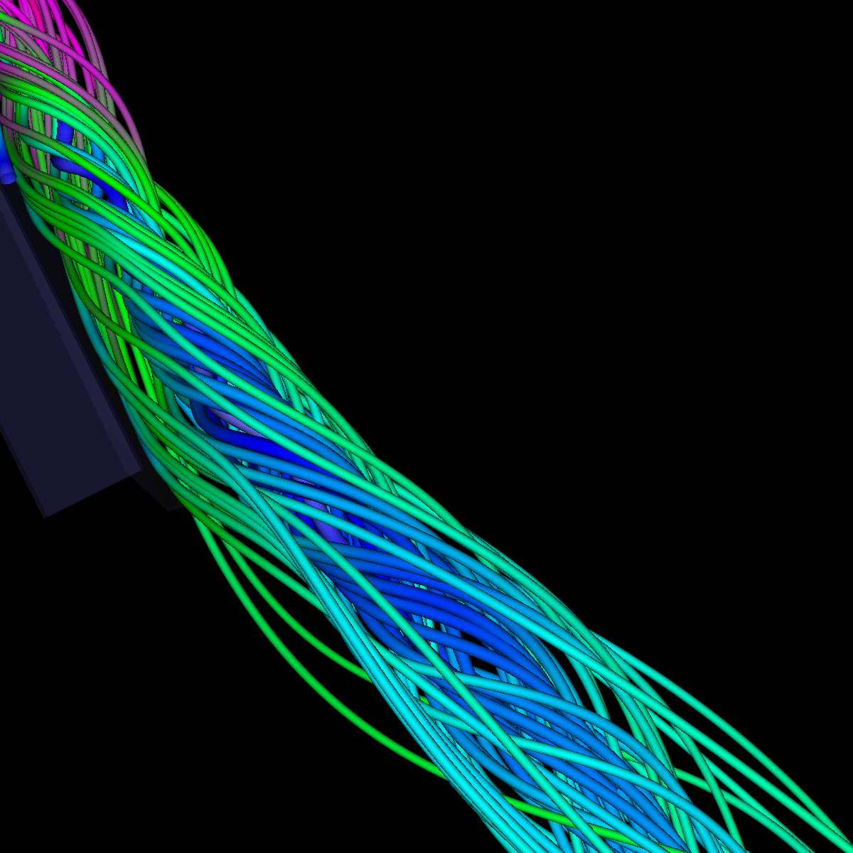 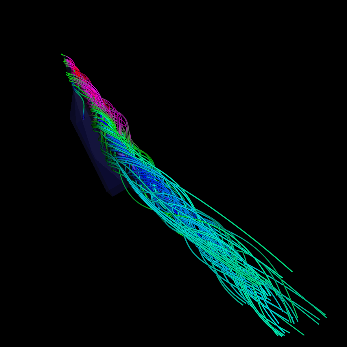 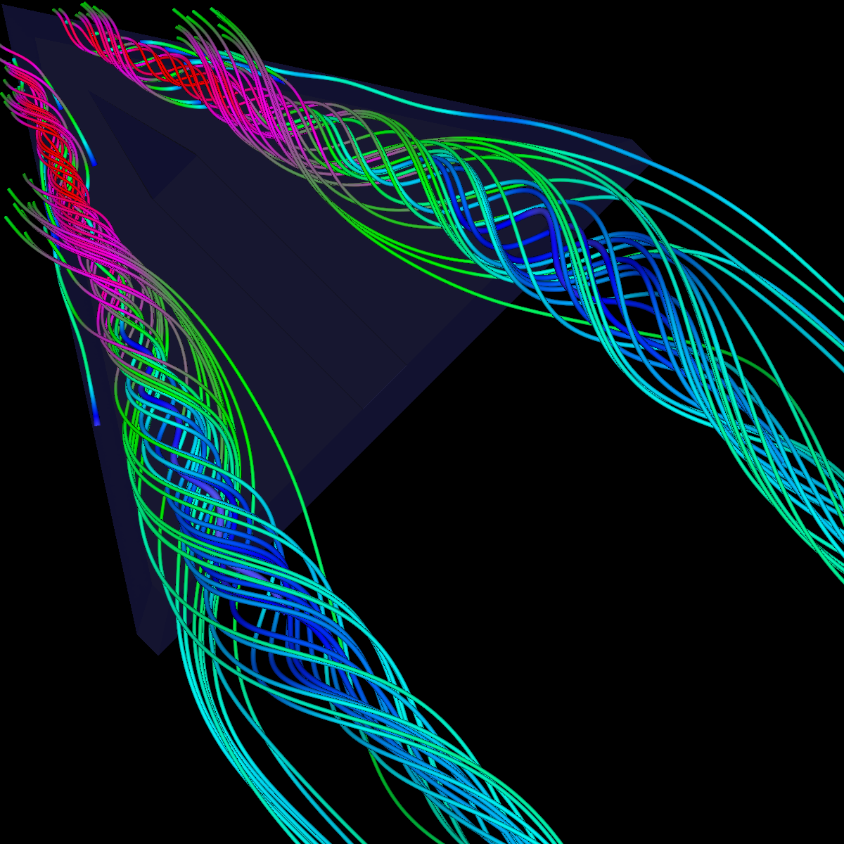 |
Part 2.3: Stream Ribbons We also visualize the flows velocity (i.e. vector field) using stream ribbons. This provides a bit more directional information that could not be captured with streamlines or streamtubes. 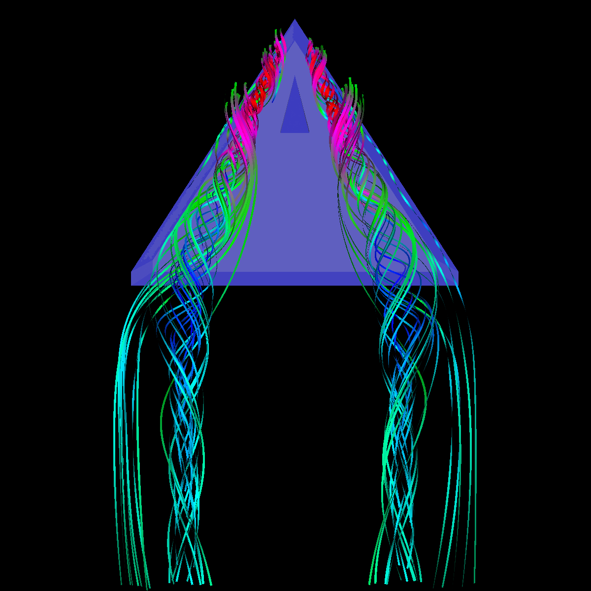 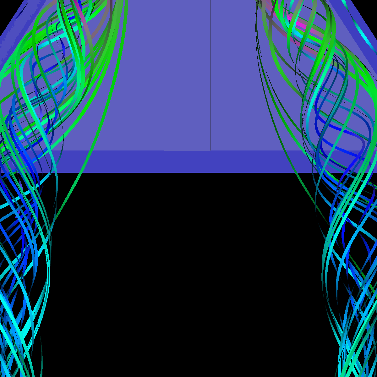 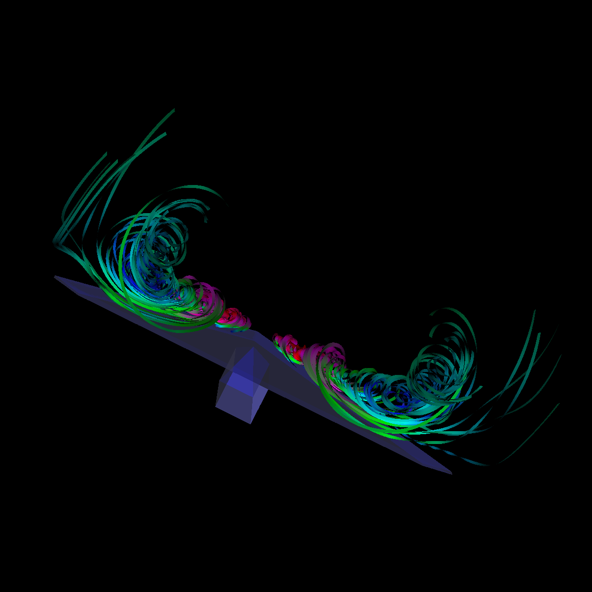 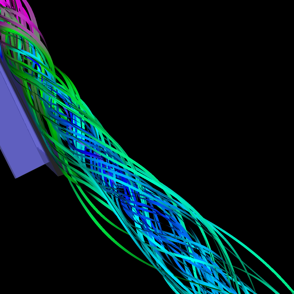 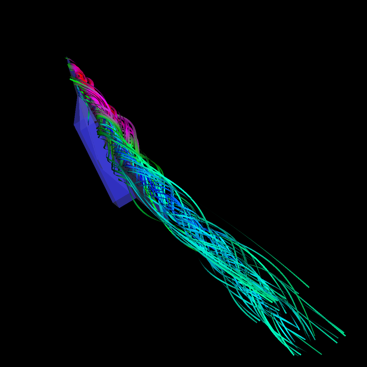 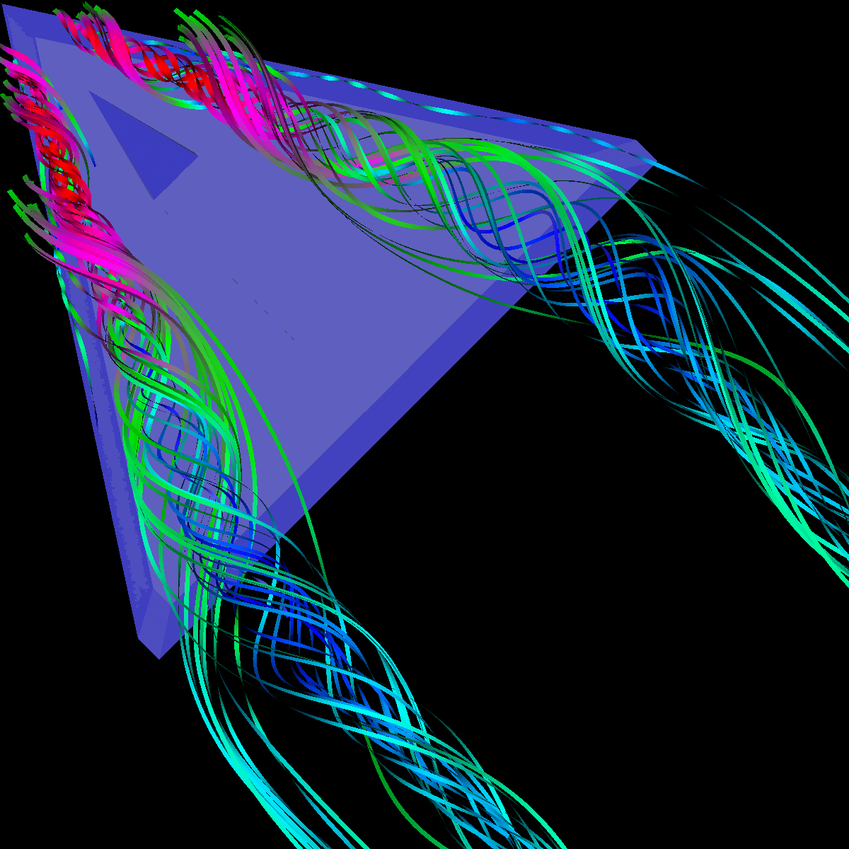 |
Part 2.4: Stream Surfaces The seeding for the stream surface was a bit more difficult since we had to randomly select seeding locations along an appropriate line. The final line was chosen using the previous intuition from sliding a clutting plane along the x-axis as well as trying many different locations until we recover the most optimal. We use forward and backward integration along the line and then stitch together streamlines with triangles to generate the stream surface. We chose seed locations randomly from the line defined by the two points (50,-40,5) and (50,40,5). We also make the stream surfaces opaque (alpha = 0.5) in order to see the inner vortices. The stream surface technique provides a unique view of the vortices that is significantly different from the streamlines/tubes/ribbons. The stream surface technique is better for capturing specific features of the vortices. For instance, stream surfaces capture the recirculation bubble extremely well as shown in Part 6. 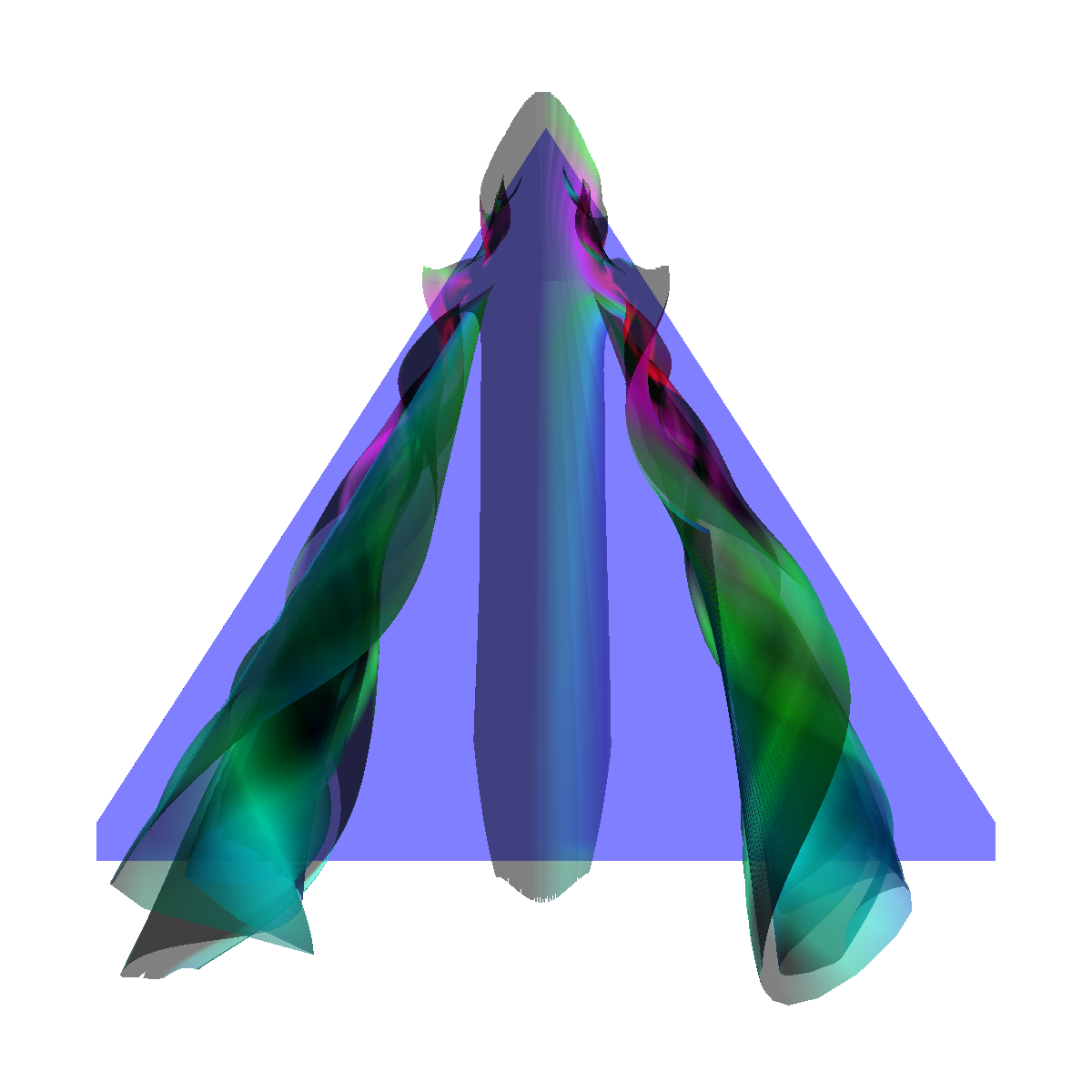 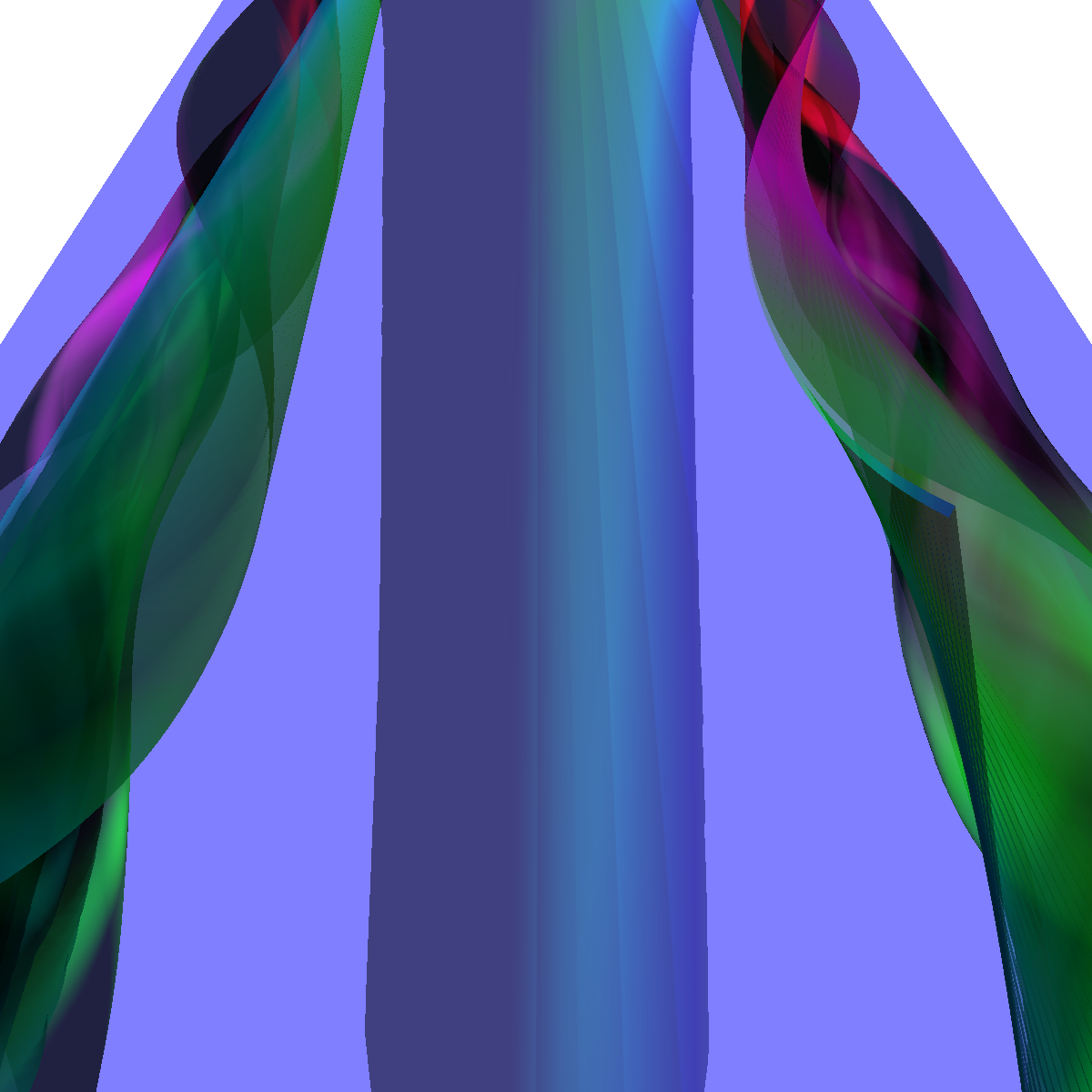 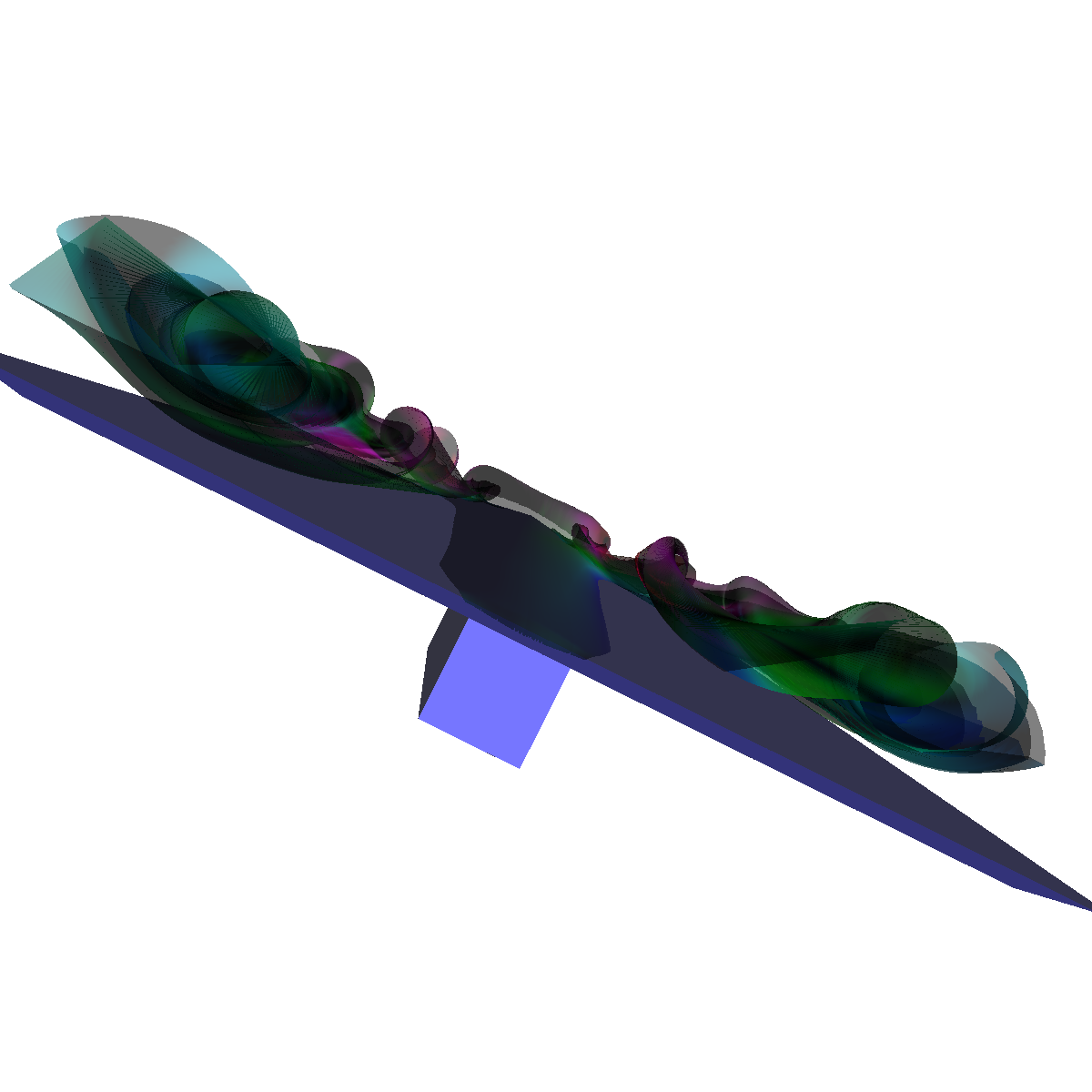 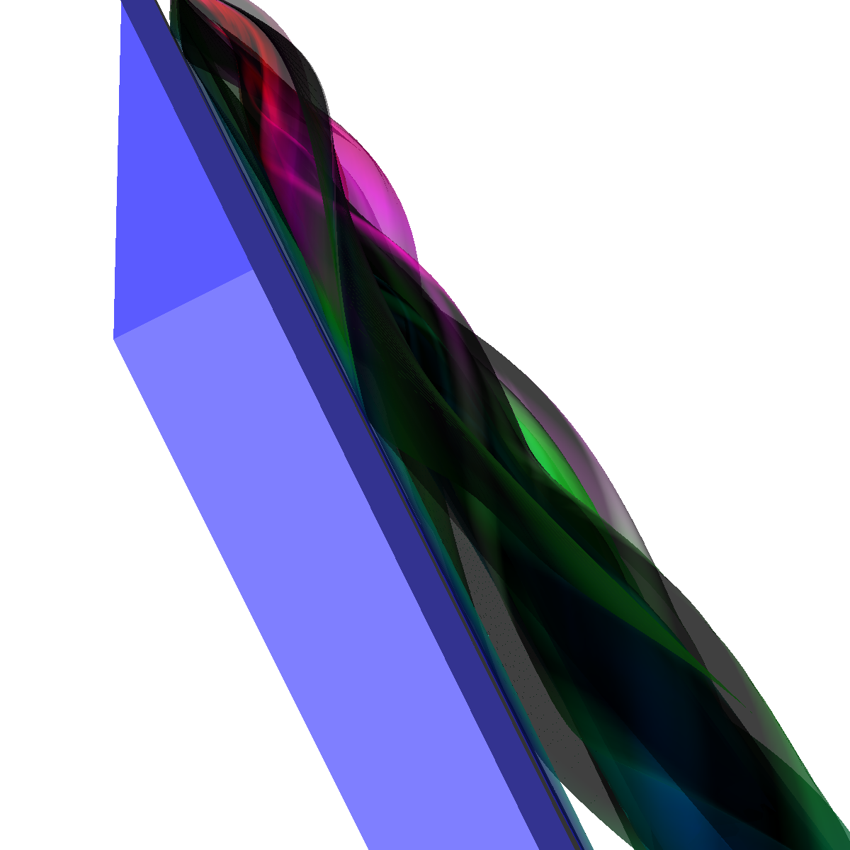 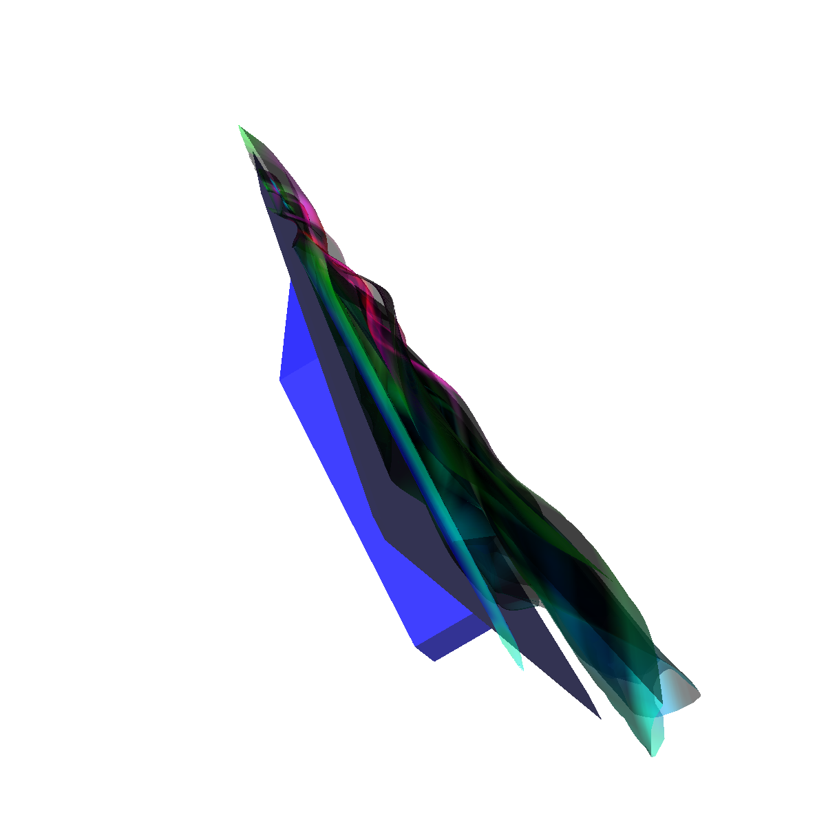 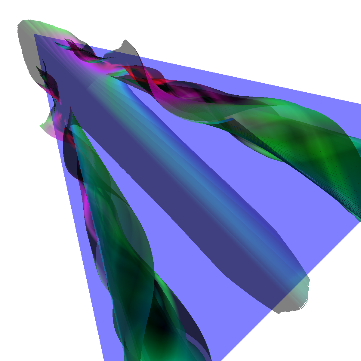 |
Part 2.4.1: Another Stream Surface In this visualization, we use another line defined by the two points (40,-40,0) and (40,40,0). We again use forward and backward integration along the line and then stitch together streamlines with triangles to generate the stream surface. 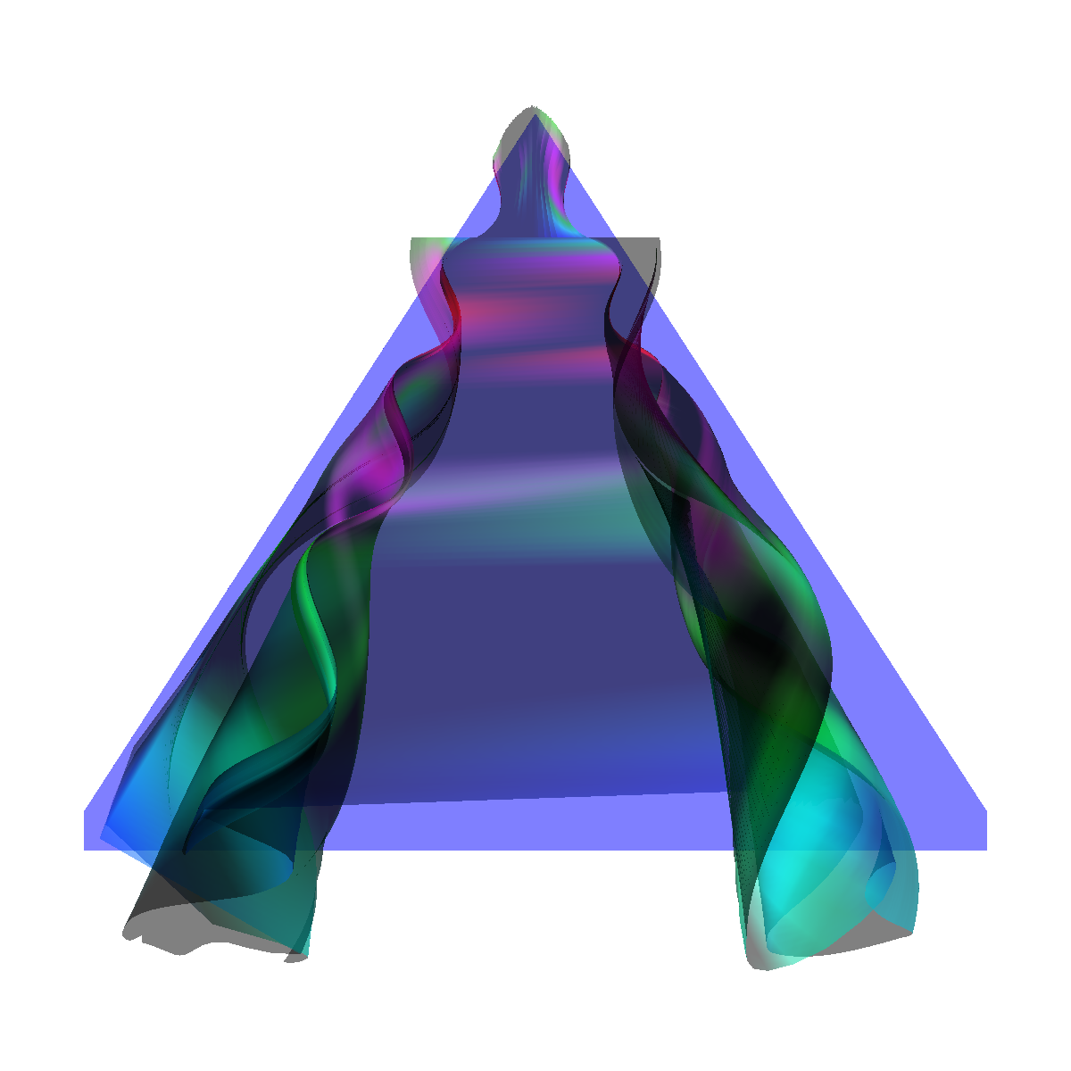 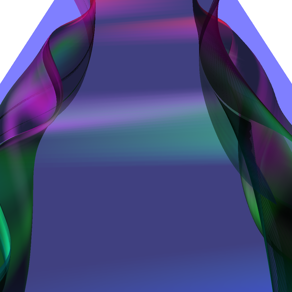 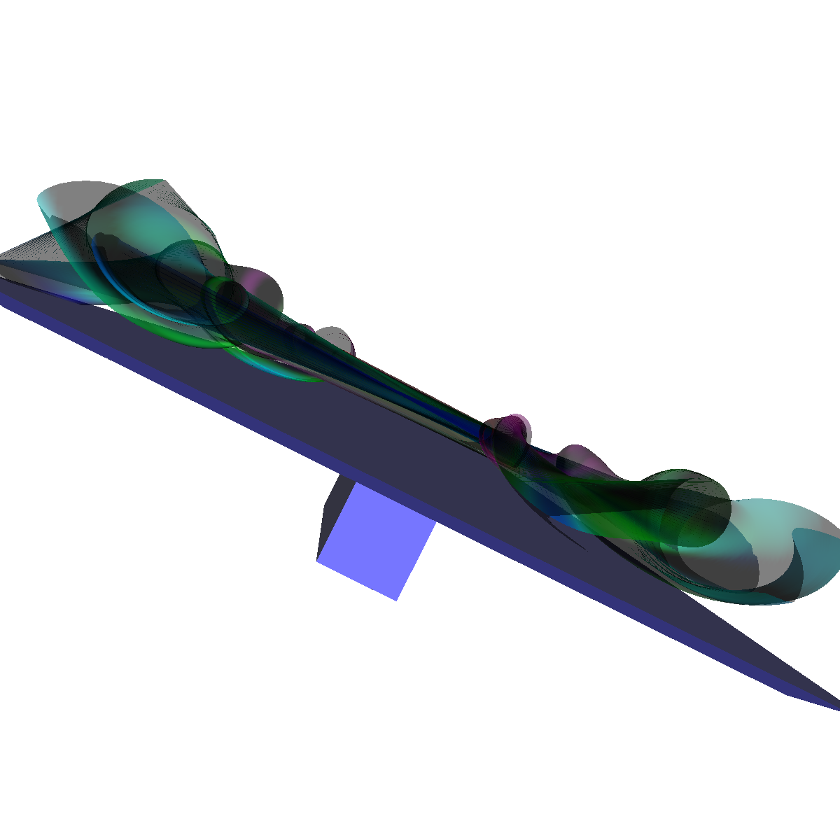 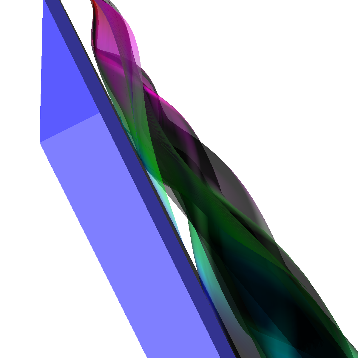  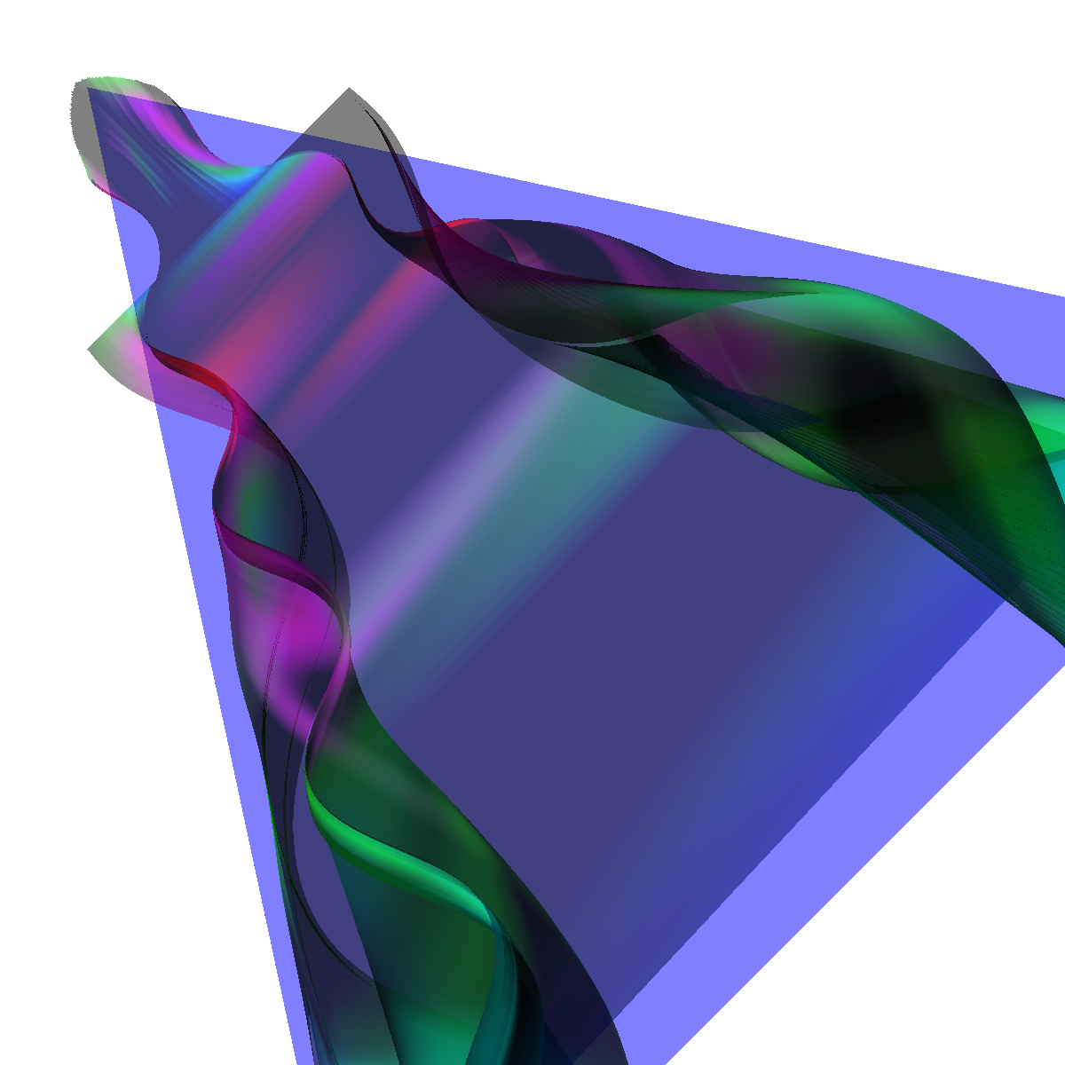 |
Part 2.4.2: Other Stream Surfaces 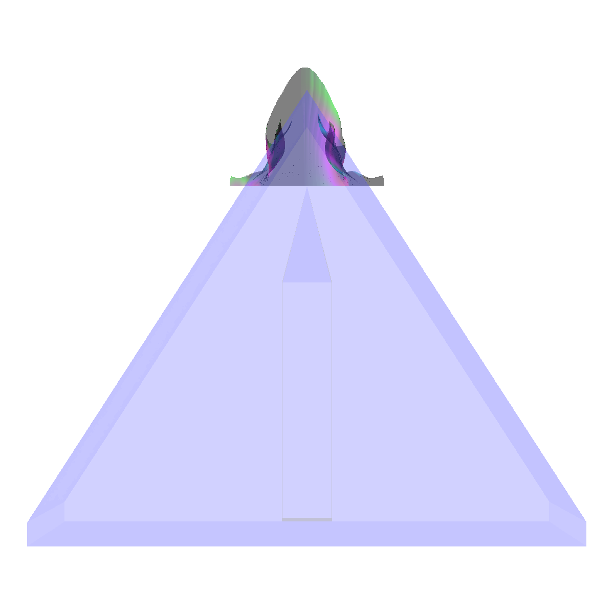 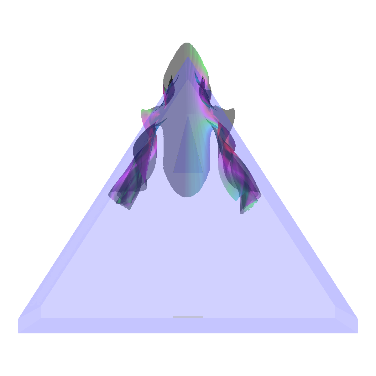 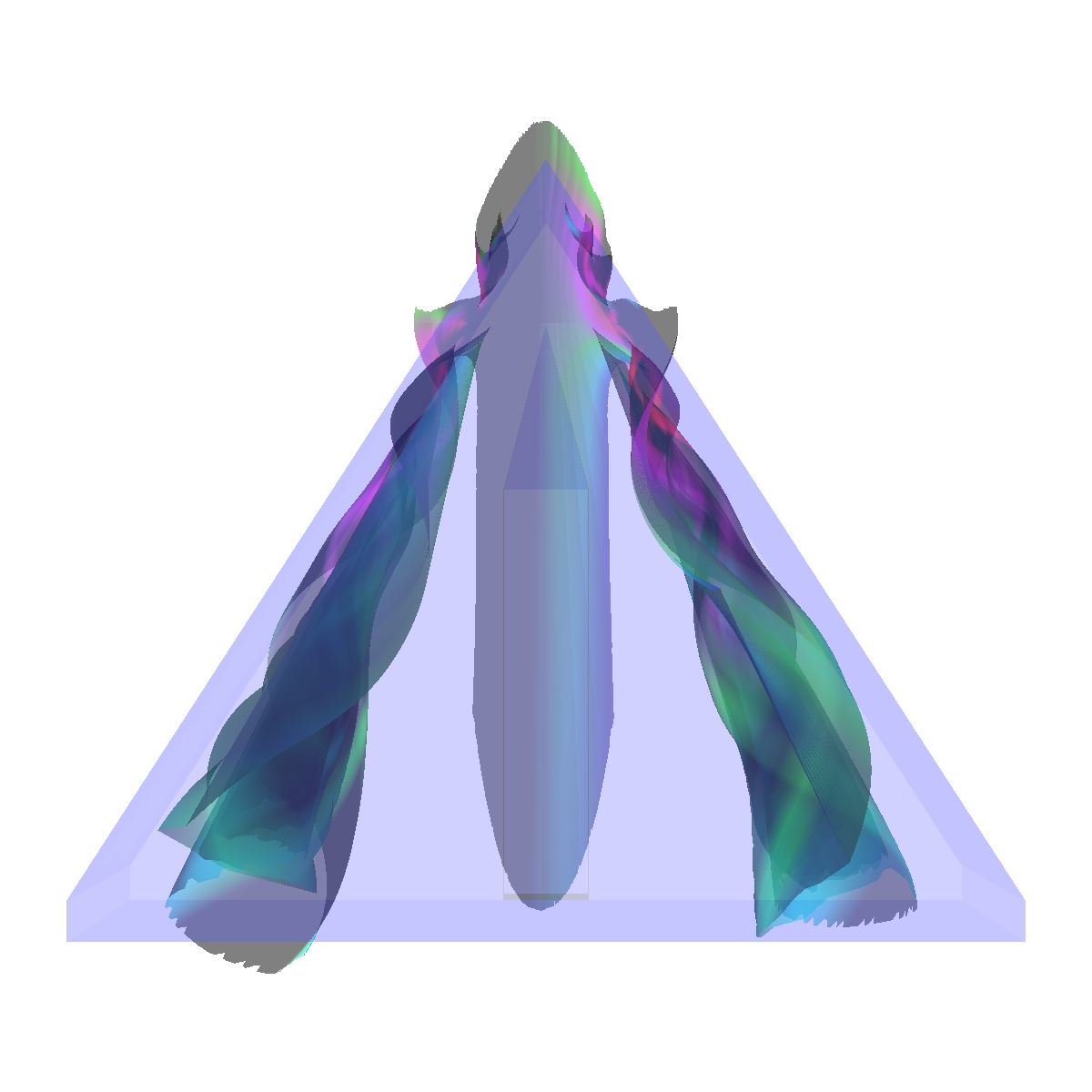 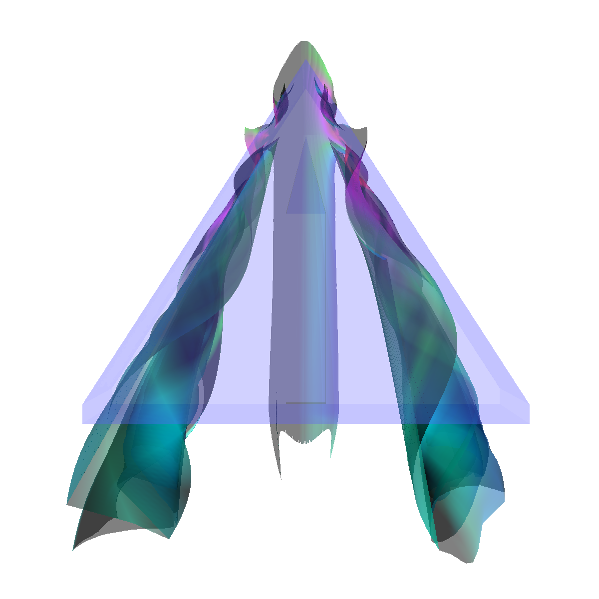 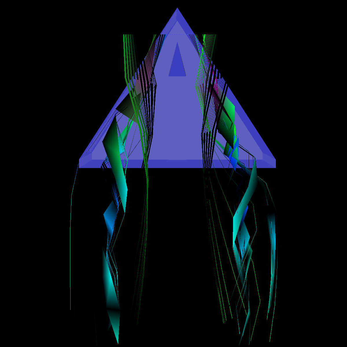 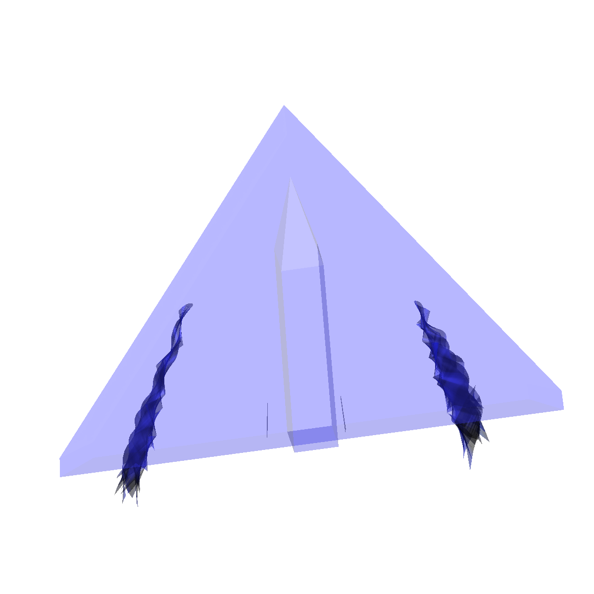 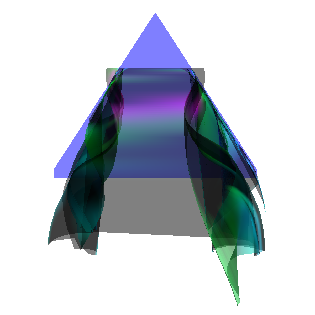 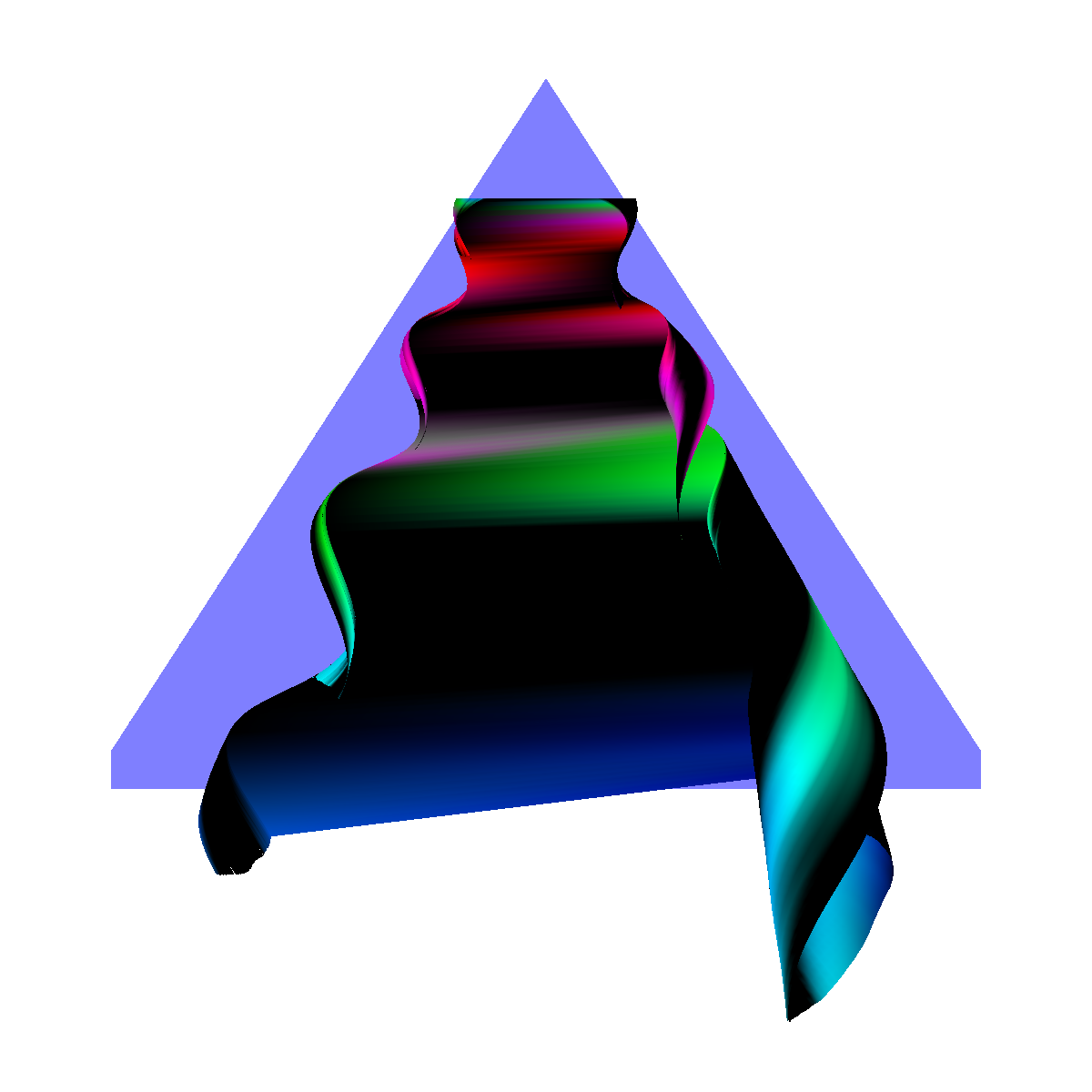 |
Part 3: Combination of Scalar and Vector Visualization We apply both scalar and vector visualization in order to capture interesting features. In particular, we use isosurfaces (scalar) and streamlines (vector field) to visualize the relationship between the streamlines geometry and the shape of the isosurfaces. Question. Describe the techniques used before arriving at the proposed solution and justify the final solution. The integration of vector visualization and isosurfacing allows for the velocity information to be visualized along side the interesting features captured by isosurfacing and conversely. In essence, we learn the velocity of a flow for a given feature at a specific isovalue (and conversely). We used this idea as a basis for the visualization below. In particular, we were interested in the flows velocity along the identified features in the isosurfacing (as shown in the visualization below). Furthermore, the complementary perspectives allow for the discovery and tuning of streamlines and eventually the corresponding isosurfaces. Both these views aid in the design of an appropriate visualization. Initially, we used the isosurface visualization previously as well as the cutting plane to define appropriate seeding locations that correspond with the isosurfaces. The isosurfacing captures many other features related to the induced vortex breakdown for which we initially did not have seed locations. Similarly, we also adjusted the isosurfacing with respect to the streamlines. We tried various approaches, such as visualizing the vector field using streamlines, stream ribbons, and stream tubes. We also tried various color maps and isosurfaces. We initially tried using a significant amount of isosurfaces in order to capture details of the vortices. However, we found using a lot of isosurfaces causes clutter and degrades from the streamlines. These observations led us to adjust various parameters including the seeding locations of our initial streamlines. The resulting visualization also aided us to appropriately visualize the recirculation bubble in part 6; as it shows up in the isosurface visualization, but lacks any interesting features or details. Furthermore, the isosurfacing provides context for the streamlines. After these observations and adjustments, we finally ended up with two isosurfaces; one with an isovalue of 50000 (blue) and another with an isovalue 55000 (red) with 0.2 opaqueness. Thus, we have a color transfer function for both the streamlines/tubes and the isosurfaces. We also combined stream surfaces, streamtubes, isosurfaces to visualize the vector field (velocity of the flow) and the scalar field. We discuss the resulting visualization and provide details in the next section (Part 3.1). Additionally, we provide a few renderings where isosurfaces are generated at different isovalues (Part 3.2). 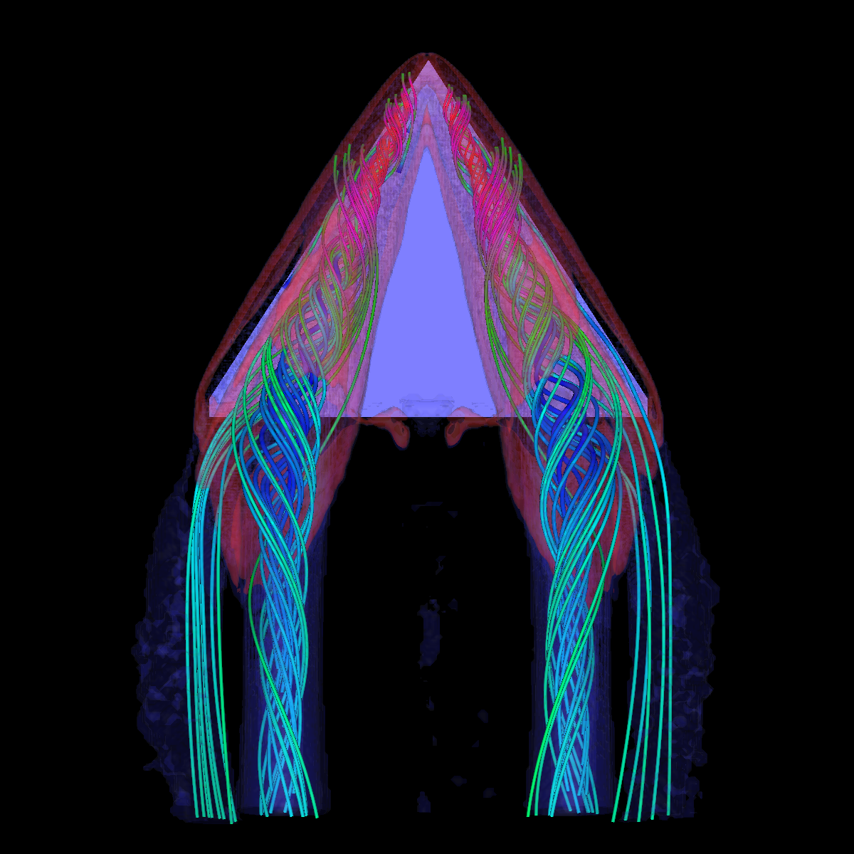 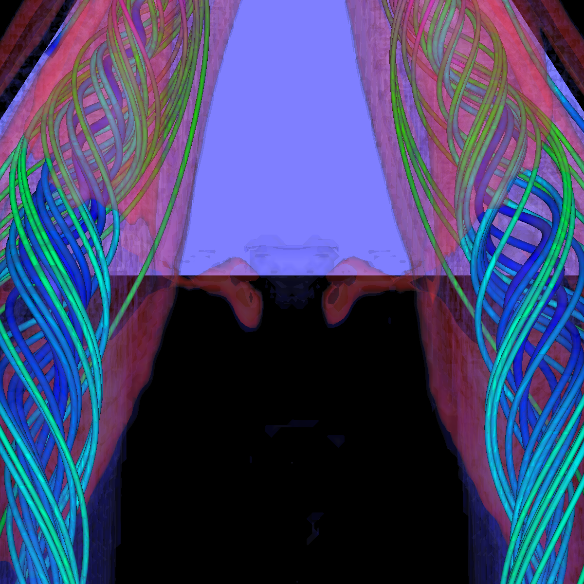 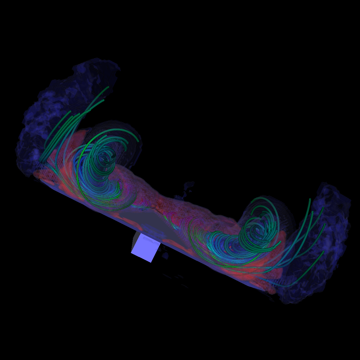 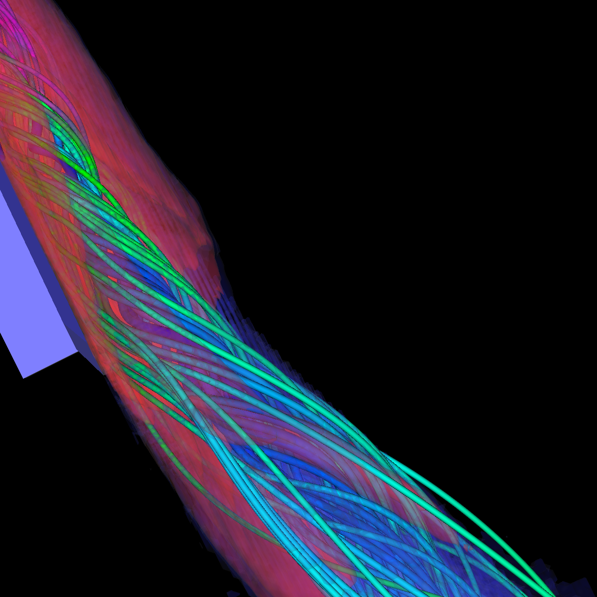 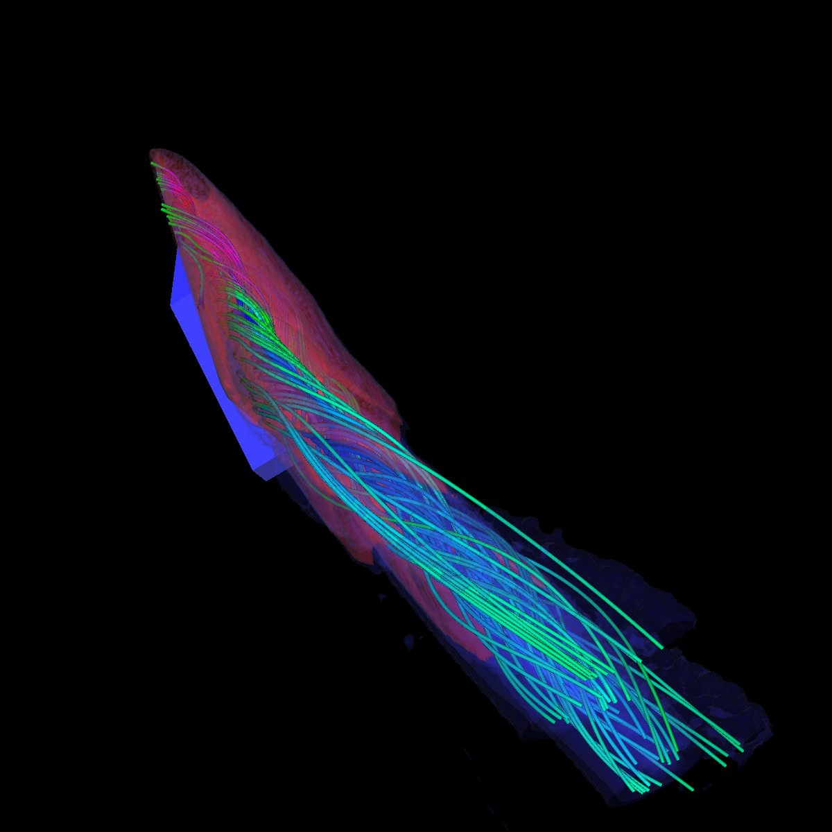 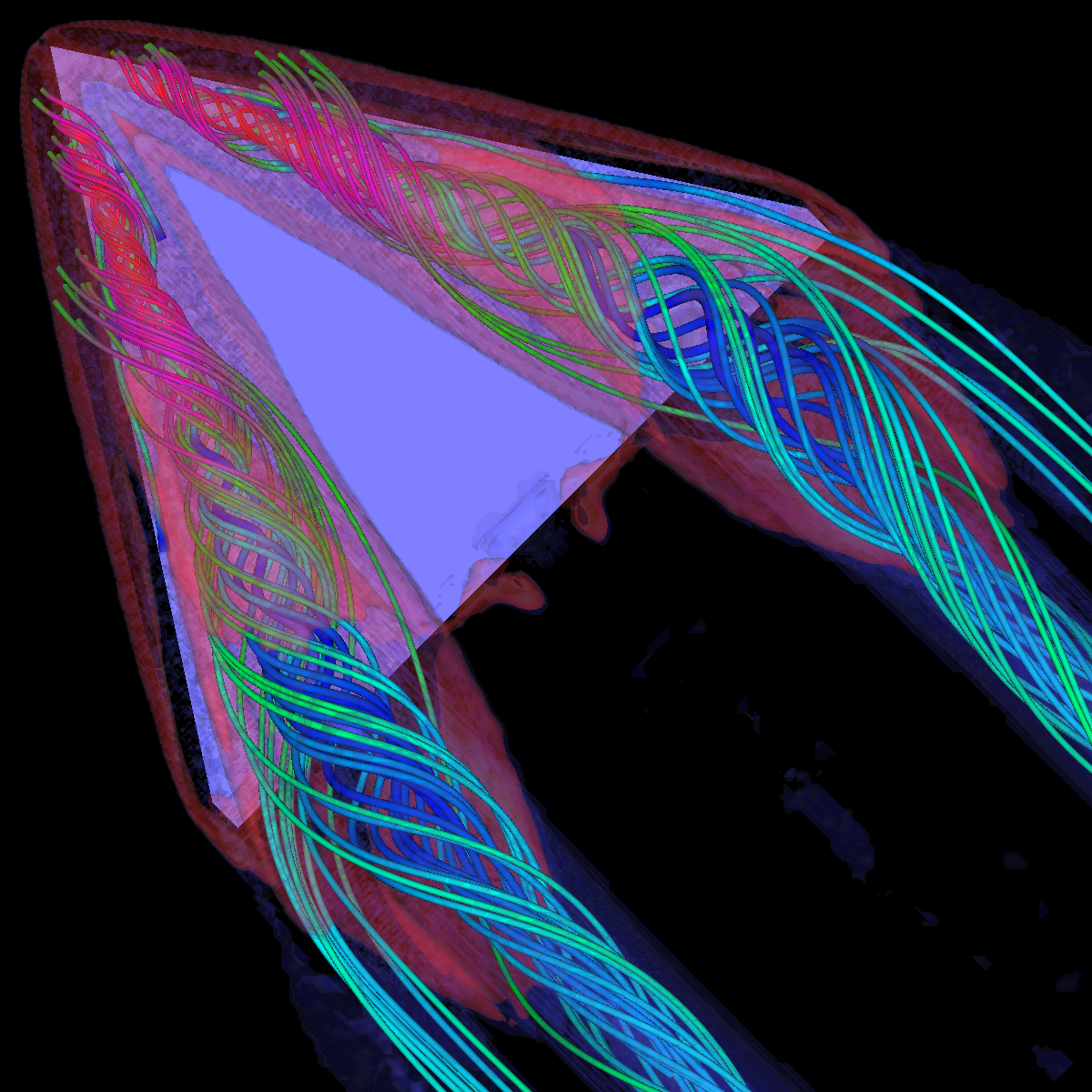 |
Part 3.1: Combination of Stream Surfaces, Stream Tubes and Isosurfaces We visualize the flow using both stream tubes and stream surfaces. The stream surfaces are defined on a line as previously specified (Stream Surfaces; Part 2.4). The stream surfaces are also opaque with an alpha=0.5. This allows the stream-surfaces and inner-vortices defined by the stream-surfaces to be viewed appropriately through the isosurfaces. 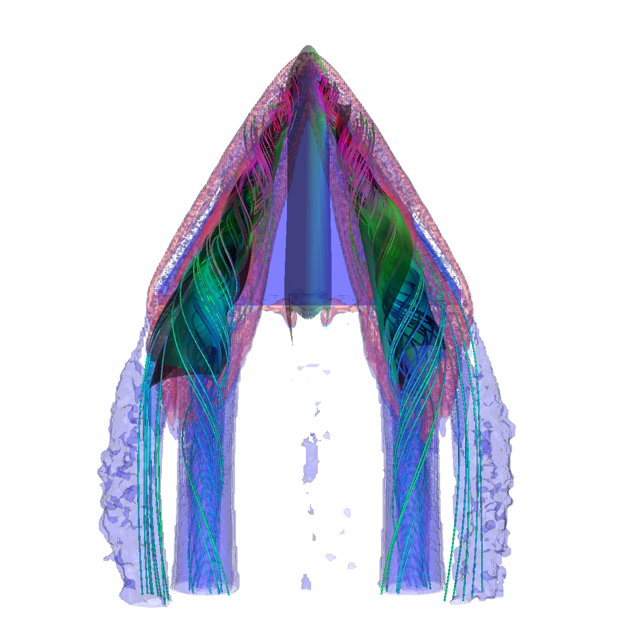 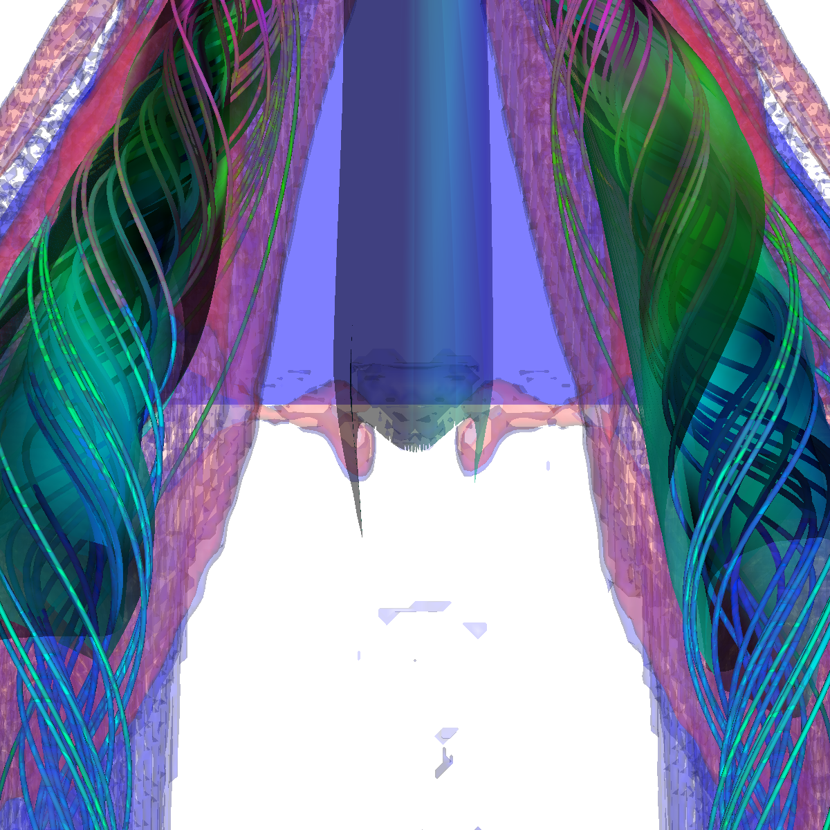 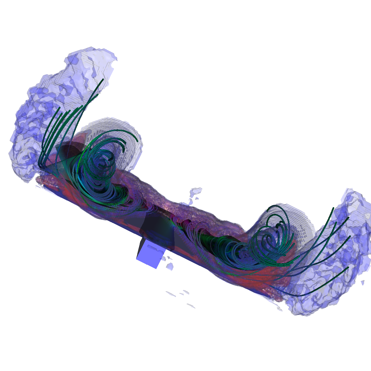 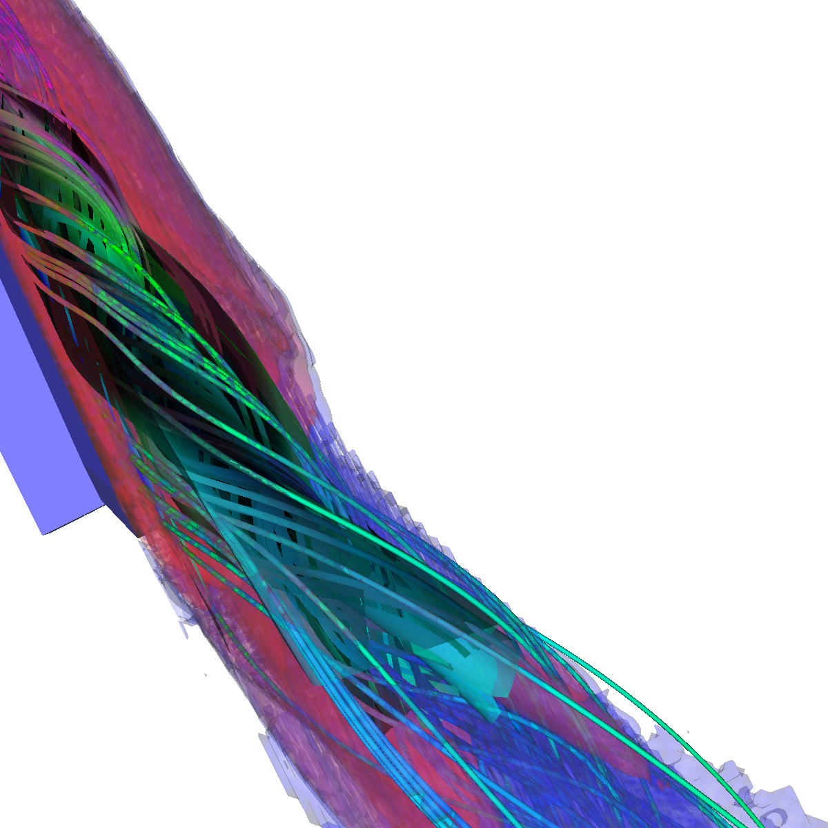 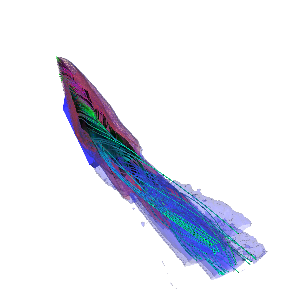 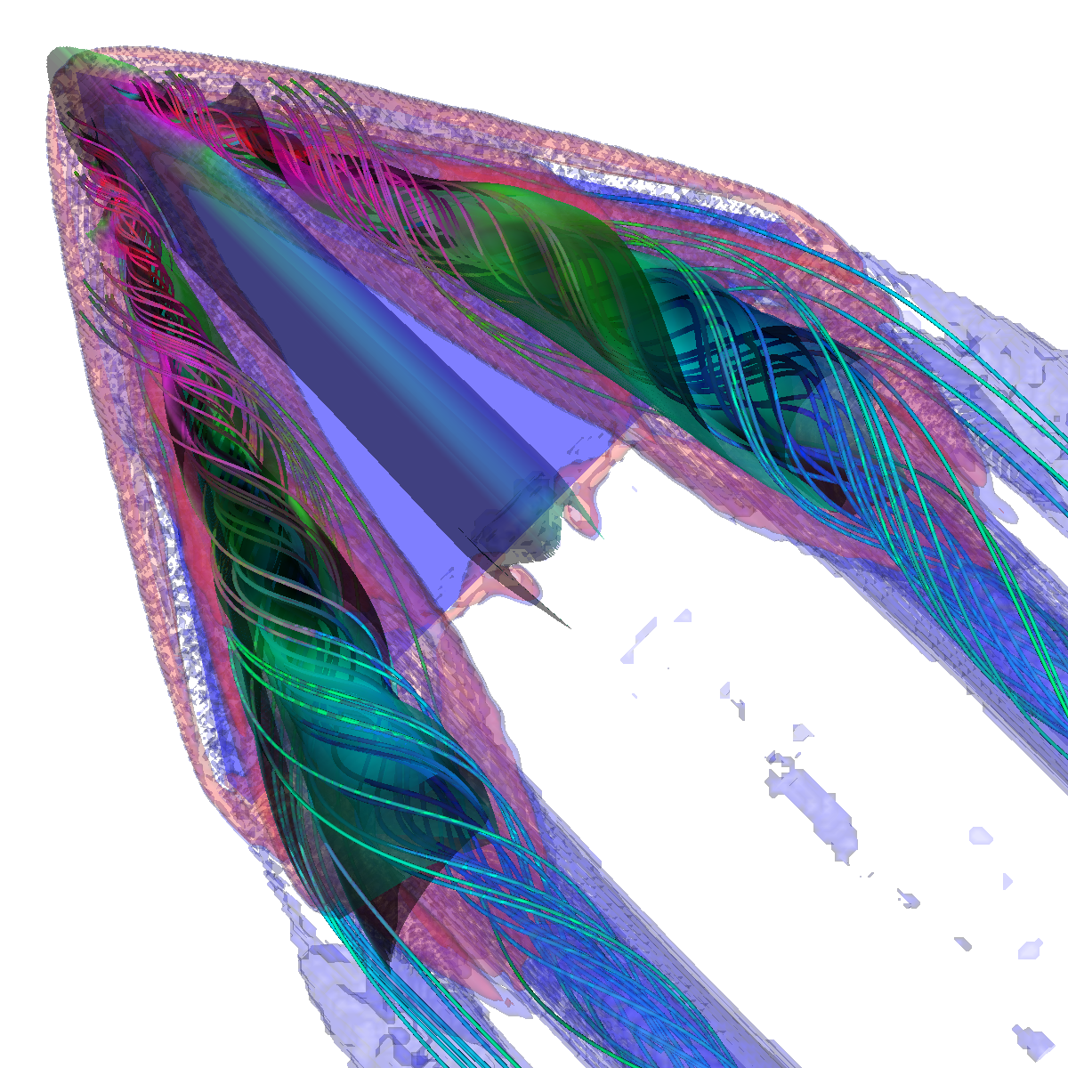 |
Part 3.2: Other Visualizations In the images below we capture the velocity information for isosurfaces generated with isovalues between 45000-60000. 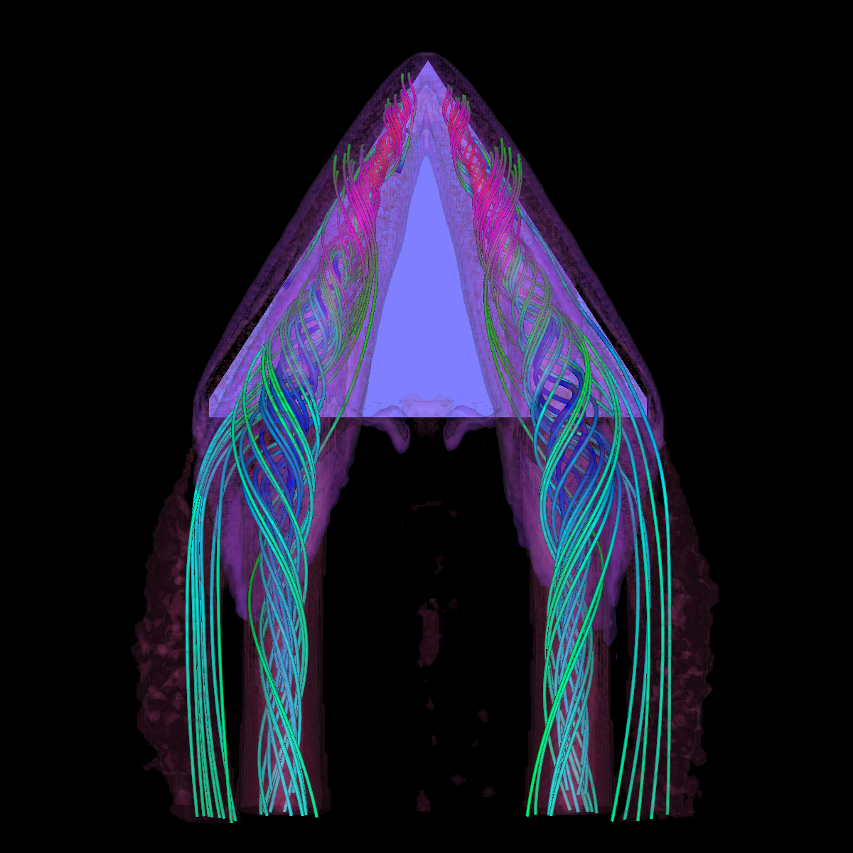 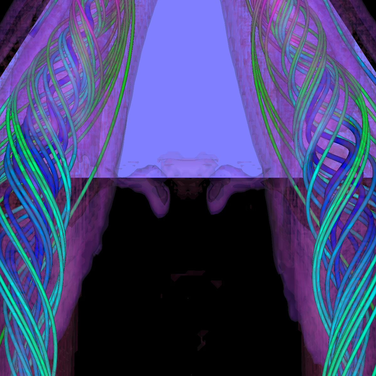 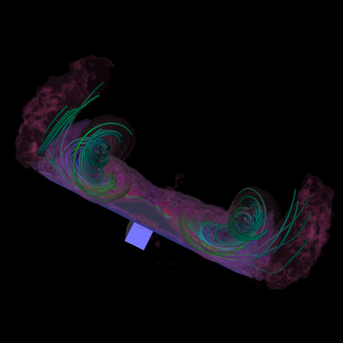 |
Part 4: Analysis We discuss and compare the previous techniques discussing the advantages and disadvantages of each. We have also discussed these techniques in detail in their corresponding sections. Part 4.1: Glyphs and Streamlines We sampled a set of planes along the vector field (velocity) and applied 3D glyphs to obtain directional information with respect to the flow. More specifically, we used arrows, cones, and cylinders to capture properties of the vector field. The arrows capture the direction and the context of the spirals whereas the cylinders fail to capture the directional information and the cones fail to capture the context but provides the direction. The glyphs along the planes provide a local view of the data and the associated features whereas the streamlines, stream tubes, stream ribbons and stream surfaces captures the global structure. Moreover, the glyphs are useful for identifying regions of interest (critical points) by locally searching the vector field. After such points are found they can be used to provide appropriate seeding locations for streamlines/tubes/ribbons and stream surfaces. Part 4.2: Streamlines, stream tubes, and stream ribbons The stream lines, stream tubes, and stream ribbons provide a more global view of the flow by capturing the direction of the flow at any point in time (instantaneously tangent to the velocity of the flow). These techniques require a selection of seed points (i.e., random cloud of points centered at a specific location with a radius to allow for variance or seeded arbitrary along a line). First, the stream lines and stream tubes provide essentially the same information, simply enlarged/scaled by wrapping a tube around the stream line. The stream tubes can be configured to vary with the vector field. However, the stream lines are useful when paired with stream surfaces to illustrate boundaries and so forth whereas the stream tubes can be bulky and detract from the stream surface. The stream ribbons are best for visualizing strong swirling along the delta wing whereas the swirling behavior is more challenging or impossible to detect using streamlines or stream tubes. The resulting visualizations (i.e., applying stream lines/tubes/ribbons or surfaces) depend upon a suitable selection of seeding locations. Part 4.3: Stream surfaces The stream surfaces are generated with a forward and backward integration along a defined line and the resulting streamlines are stitched together with triangles. Choosing an appropriate seeding location is generally difficult, especially without domain knowledge. Stream surfaces proved to be the most appropriate technique for capturing the recirculation bubble and the corresponding properties (as shown in Part 6). The stream surfaces are even more difficult to use as the parameter space and possible visualizations is substantially increased from the space of visualizations from stream lines. For instance, we must not only choose the appropriate step length in order to appropriately capture the vortices and the interesting features (i.e., flow and swirling patterns; as is selected for streamline visualization), but we must now select various other parameters such as resolution if we apply resample and also a distance factor and if we walk and stitch using the points then we must set the distance factor. Furthermore, an appropriate opaqueness (alpha value) must be chosen in order to see the inner features of the stream surfaces. Nevertheless, every choice might drastically impact the resulting visualization. Clearly, an individual must both know a lot of underlying details on how the algorithms work and their impact in 3D space as well as having plenty of domain knowledge for selection of not only seeding locations but opaqueness, among others. Part 4.4: Combination of vector visualization and isosurfacing The combination of vector visualization techniques (streamlines, stream tubes, stream ribbons, stream surfaces) and isosurfacing provide a unique opportunity for interesting visualizations. The integration of vector visualization and isosurfacing allows for the velocity information to be visualized along side the interesting features captured by isosurfacing and conversely. In essence, we learn the velocity of a flow for a given feature at a specific isovalue (and conversely). Moreover, the isosurfacing provides context for appropriately including the stream lines . In particular, the isosurfaces aid in the design of the vector visualization as a more global static view is specified at every isovalue. Therefore, based on this, seeding locations for visualizing the velocity can be chosen such that the streamlines go through or near the features captured in the isosurface. For instance, we initially failed to capture the structures on either side of the wing using vector visualization, but were able to place streamlines in such a way to clearly visualize the velocity for these features or regions. The reverse also applies, in that stream lines could be used to aid in the design or selection of an isovalue or transfer function, but it is of lesser significance. |
Part 6: Visualization of Flow Recirculation Question. List the techniques applied and discuss the reason for certain choices. We visualize the recirculation bubbles associated with the vortex breakdown phenomenon. The recirculation bubble is best captured by combining visualization techniques. In particular, we used stream lines, stream tubes, stream ribbons, and stream surfaces. We also used the glyphs with a cutting plane and isosurfaces in order to locate and isolate the recirculation bubbles. We had trouble completely isolating the recirculation bubble as we ran into video memory issues as we decreased the step size to a length where we could clearly see the unique vortex breakdown features. Nevertheless, we are able to capture most of the recirculation bubble. The recirculation bubbles are first captured by selecting the critical point associated with the vortex breakdown structure. After we identified the critical points, we visualize the recirculation bubbles by applying stream surfaces and stream lines. We can also use stream ribbons or stream tubes to highlight significant features within the recirculation bubble by first assigning the recirculation bubble with an appropriate opaque value in order to visualize the features inside as the bubble wraps around and grows. In part 6.1, we apply isosurfaces, glyphs, as well as stream lines, stream ribbons, stream tubes, and most importantly stream surfaces. In the next section, we apply stream surfaces, stream lines, and stream tubes to capture the recirculation bubble (Part 6.2). We find that the features of the recirculation bubble are visualized best using stream surfaces and stream lines. In part 6.2, we experiment a lot by changing various parameters including integration schemes, distance factors, critical point locations, seeding locations, and many others. |
Part 6.1: Stream Surfaces and Isosurfaces for Visualizing the Flow Recirculation Question. Discuss the techniques applied and the reason for certain decisions. We visualize the recirculation bubble by first choosing an appropriate line at location (180,120,5) to (180,-120,5) and applying stream surfaces (alpha=0.15), streamlines, and stream ribbons. We then use the previous isosurface and stream tubes for context. We generated the stream surface, stream ribbons and streamlines along this line. The line was chosen for the stream surface in an attempt to capture the beginning of the vortex breakdown structure. The isosurface clearly shows the ends of the structure and the vector visualization provides the corresponding velocity information. 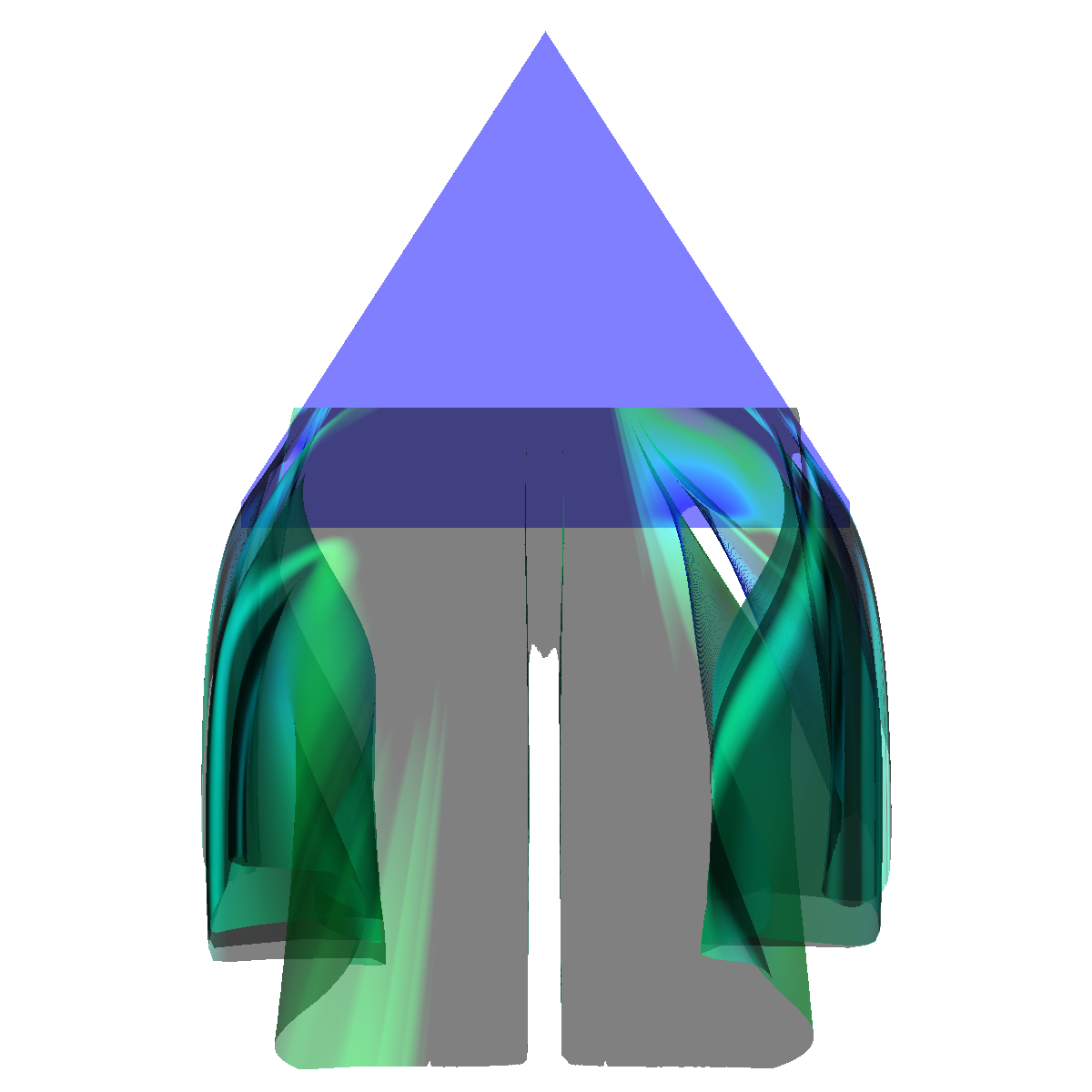 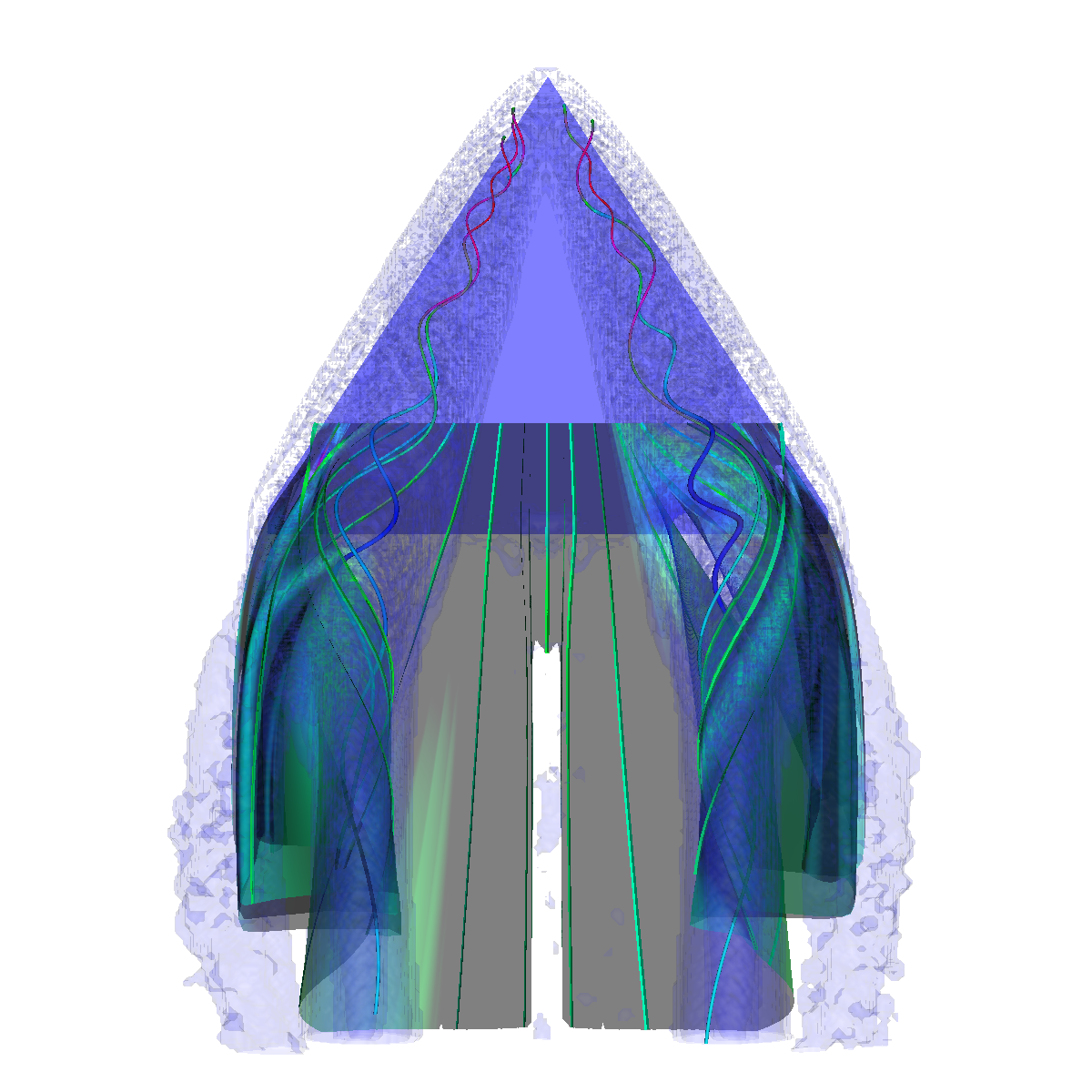 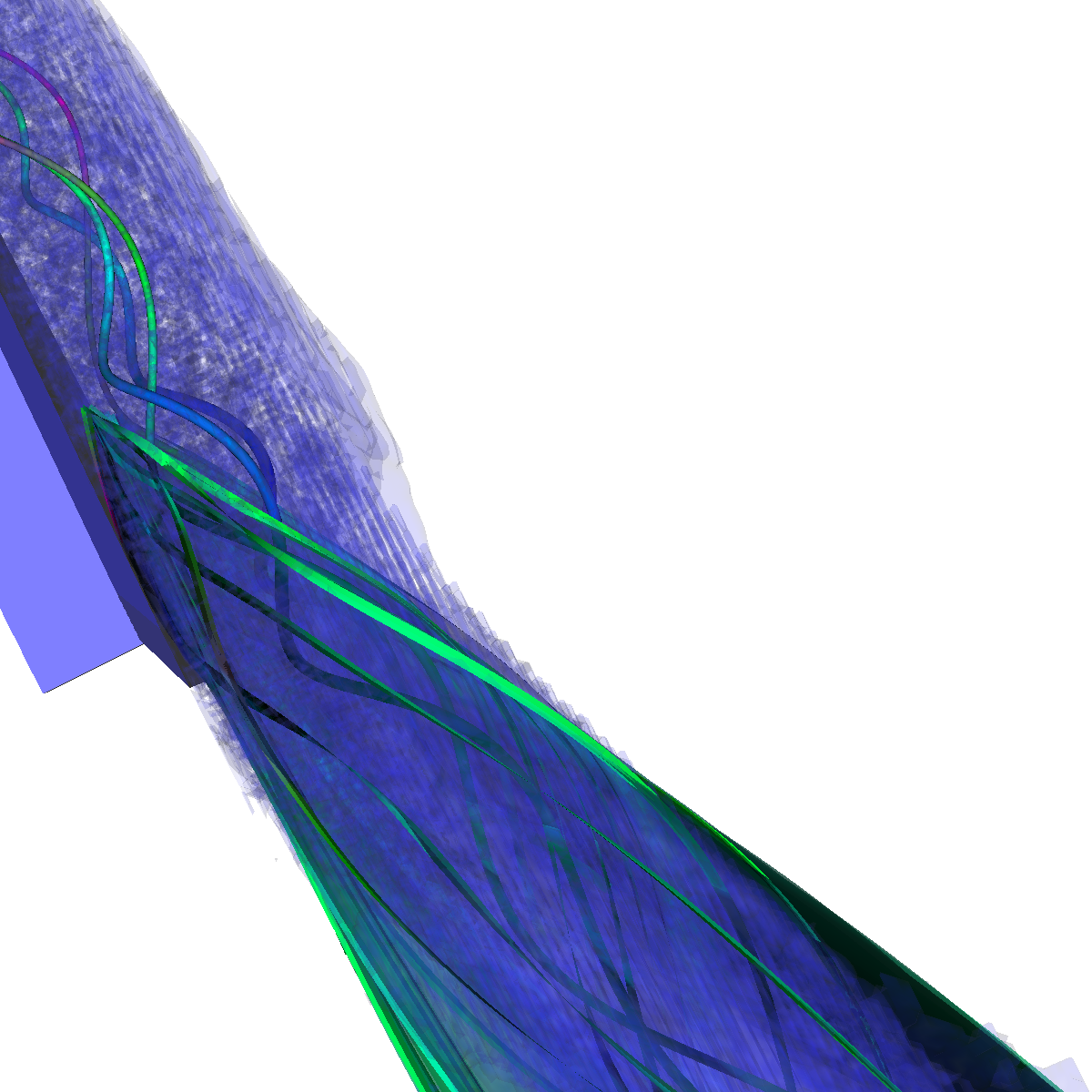 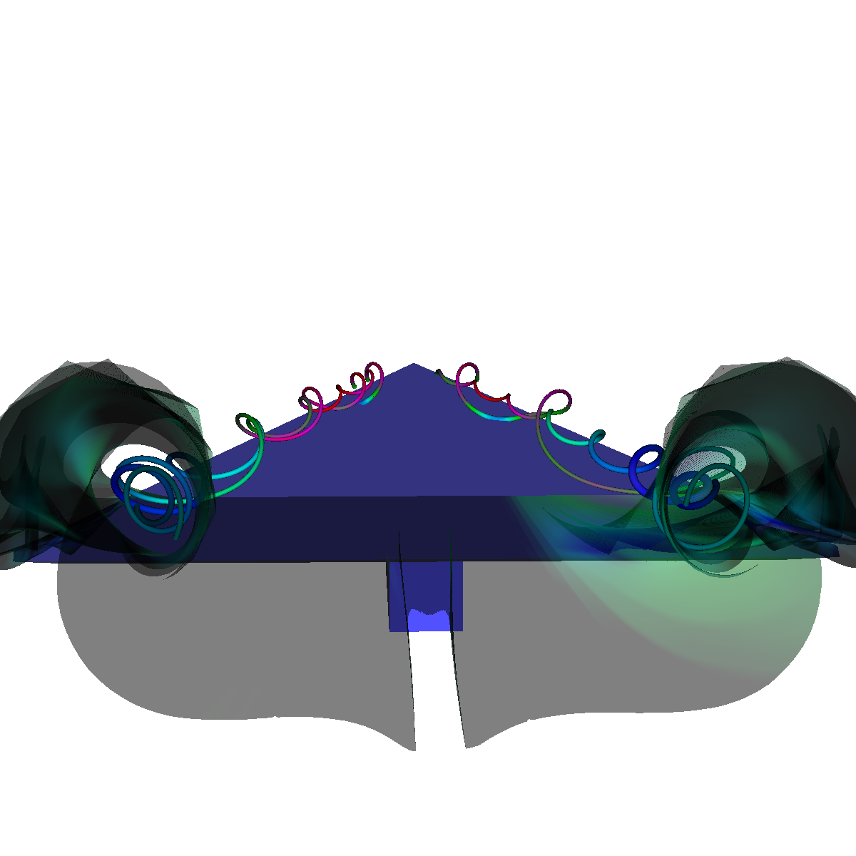 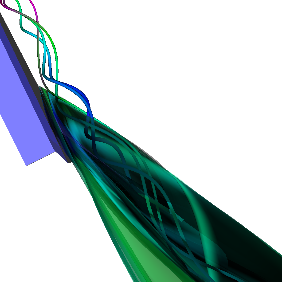 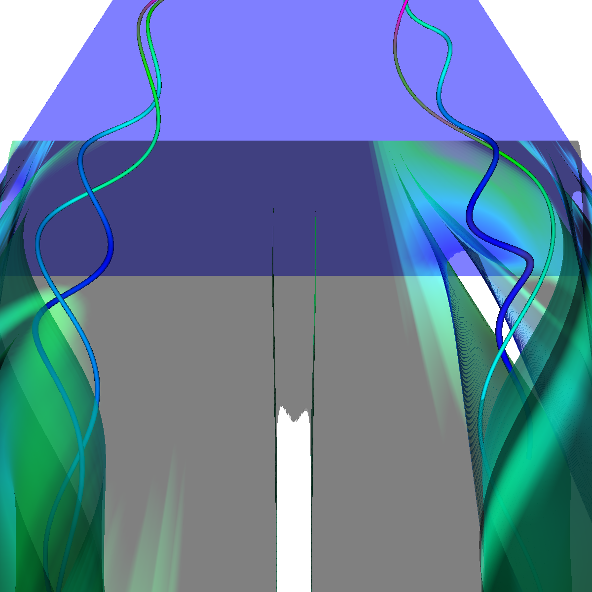 |
Part 6.2: Visualizing the Recirculation Bubble using Stream Surfaces, Streamlines, and Stream Tubes Question. Discuss the techniques applied and the reason for certain decisions. In the next sections, we use stream surfaces as a basis along with stream lines, and stream tubes (for context) to visualize the vortex breakdown and the interesting features. We apply transparency (alpha=0.15) to the stream surfaces and stream lines and use the previous color coding. For the stream surface, we placed a rake (line source) at various locations (defined precisely, in each section). The rake was placed at this location as it corresponds to one pair of critical points (one at each side of the wing) that eventually lead to the formation of the recirculation bubble. The other major critical point which is hardly of interest is the center (2,0,0) of the plane where the flow is smooth over the wings (as seen in Part 1). We also tried seeding the stream surface by randomly selecting points up to a specified radius around a center point. The intuition was that this would generate many stream surfaces embedded in one another. The next sections discuss further the intuitions for each approach. We had memory issues as we attempted to set the length of the streamline integration to a low enough value to capture all the minor details of the recirculation bubble. Nevertheless, we were able to visualize the majority of the features associated with the vortex breakdown. Below we show a few of the visualizations. 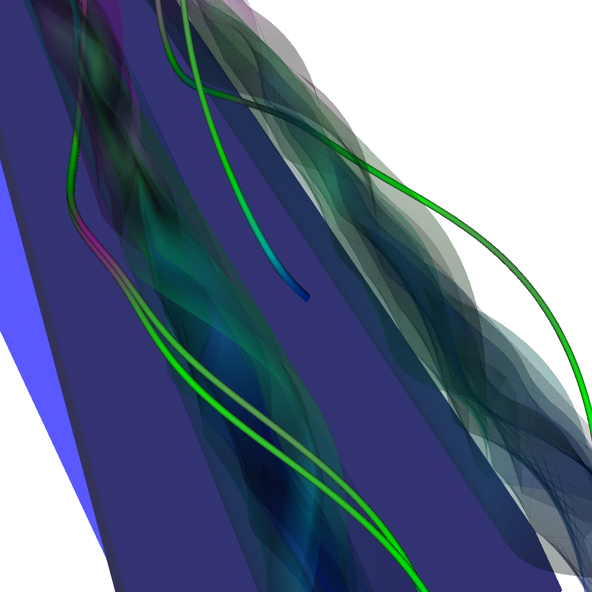 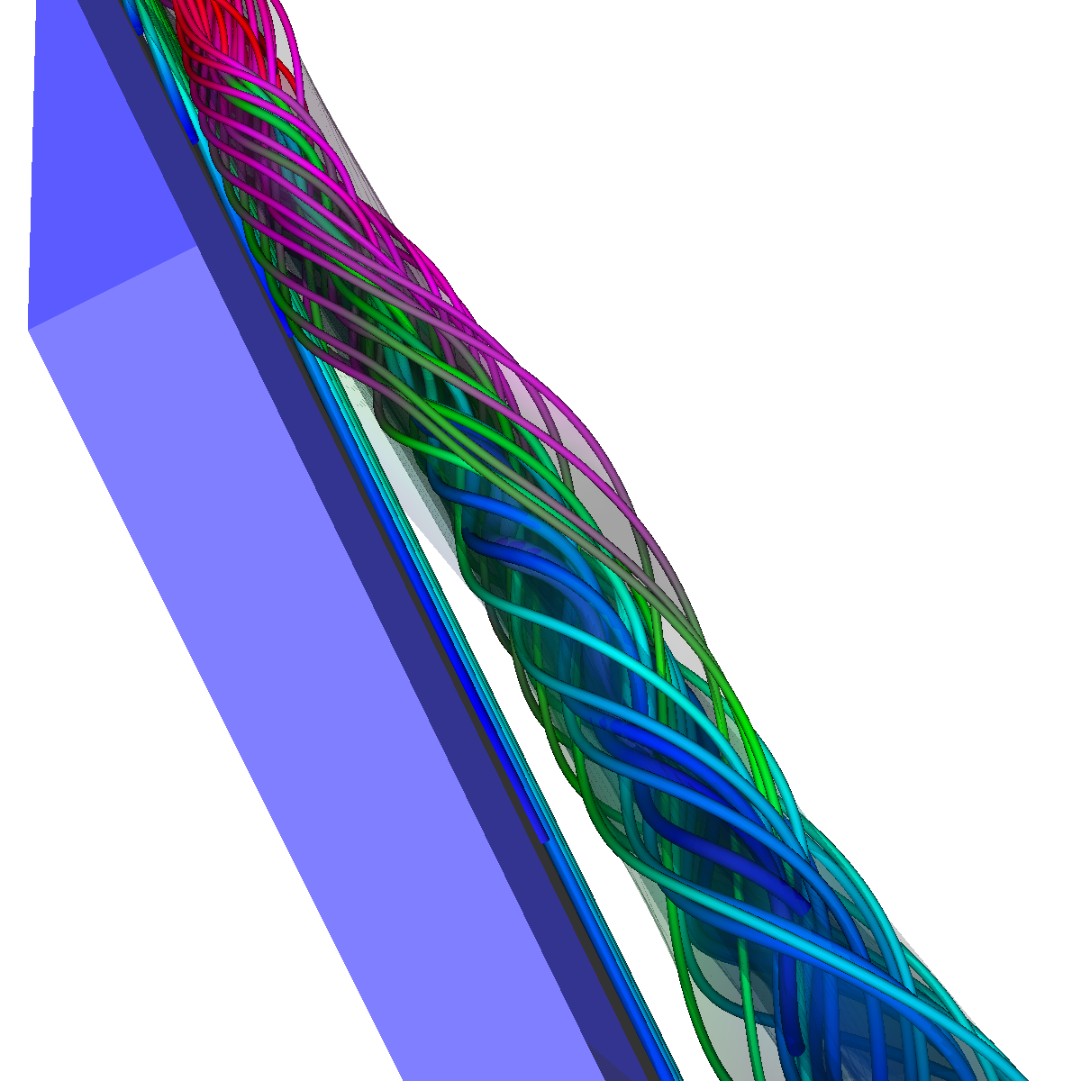 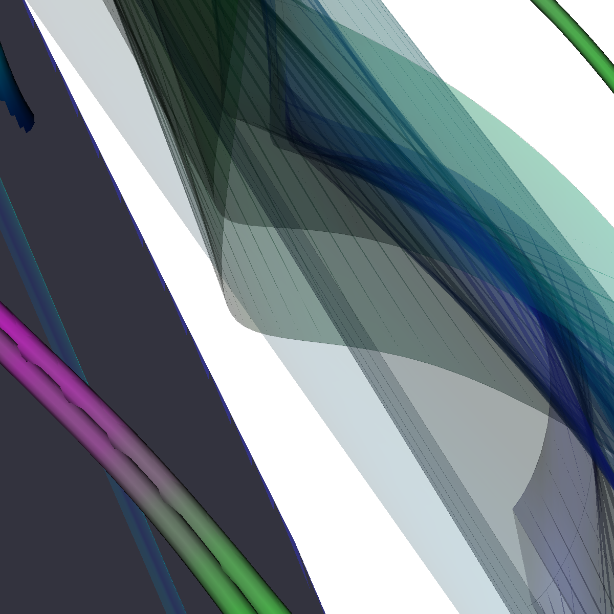 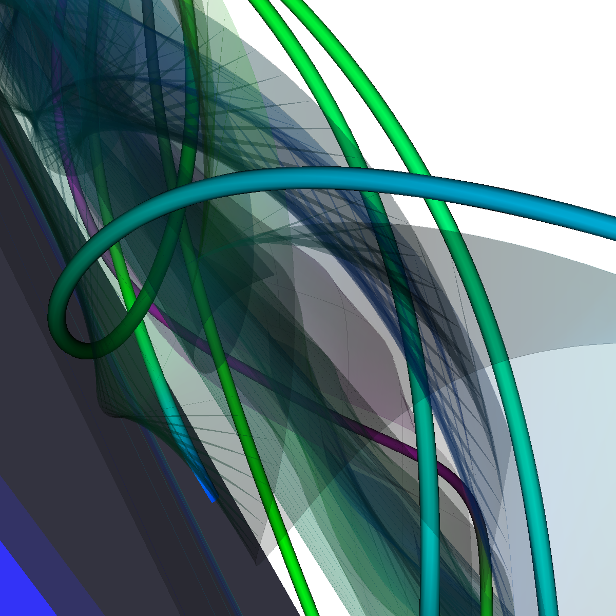 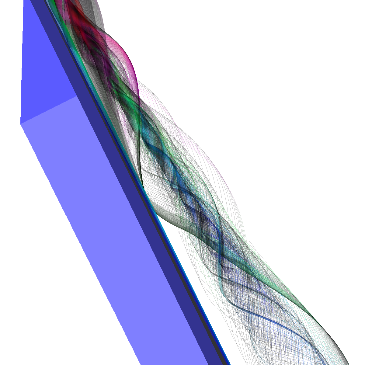 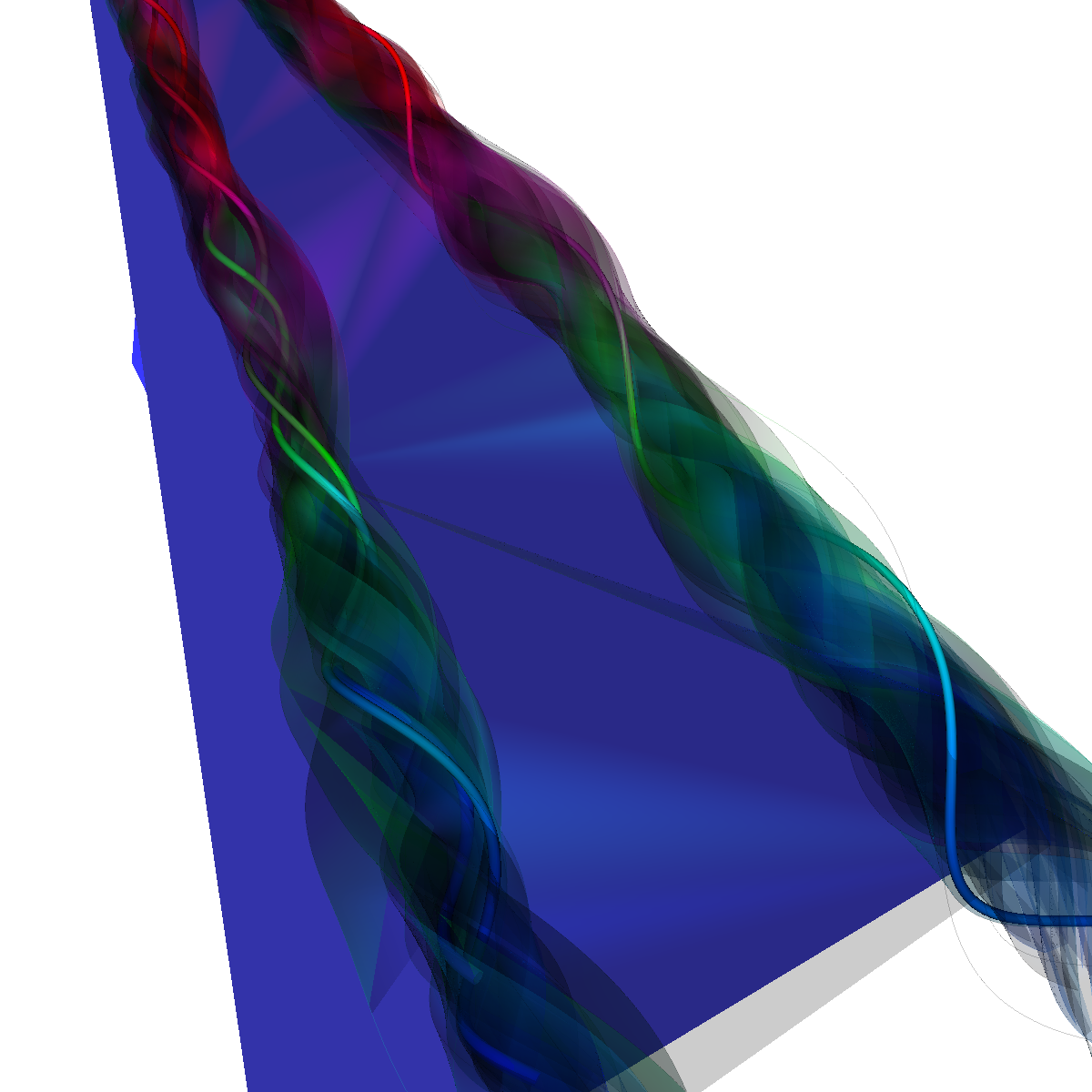 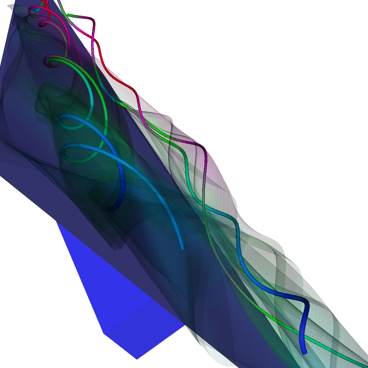 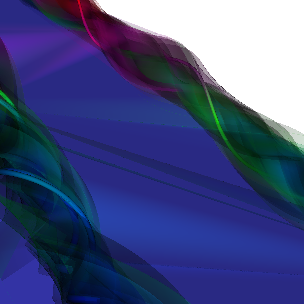 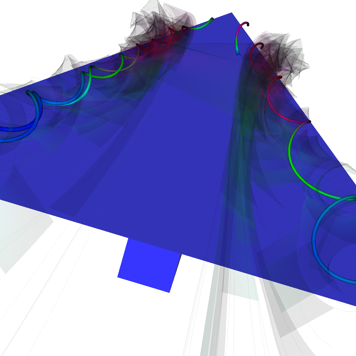 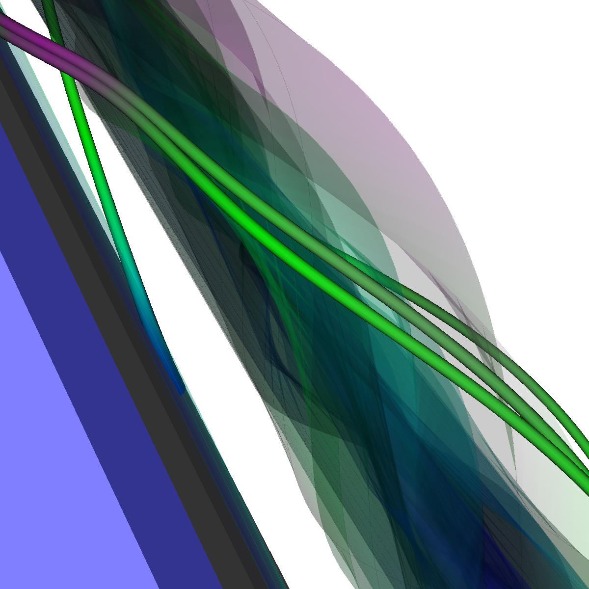 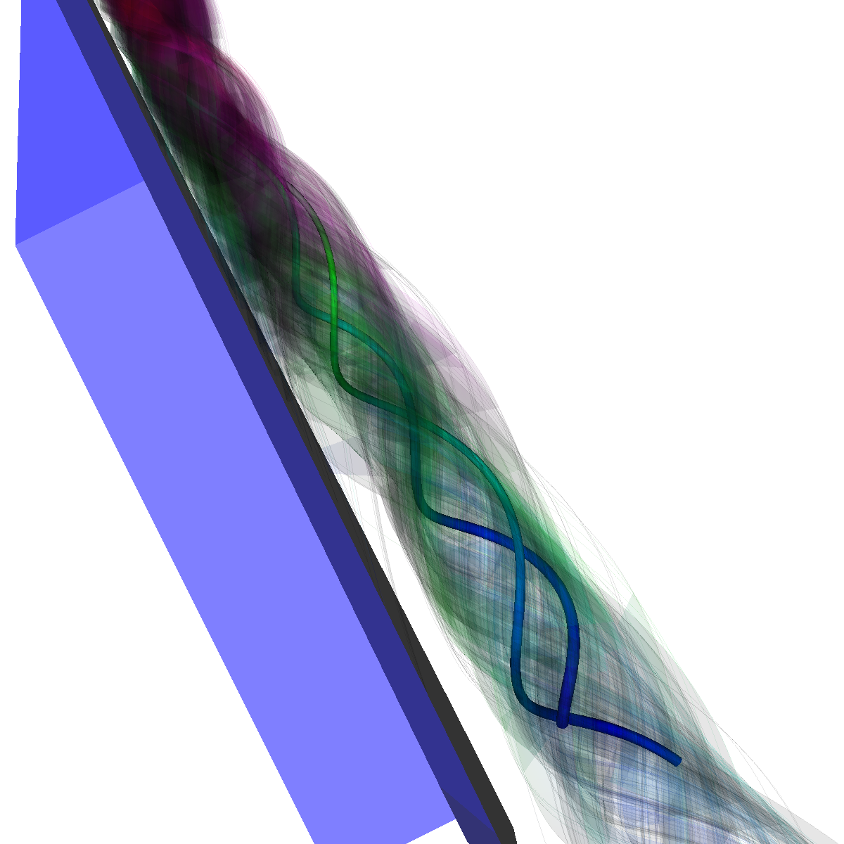 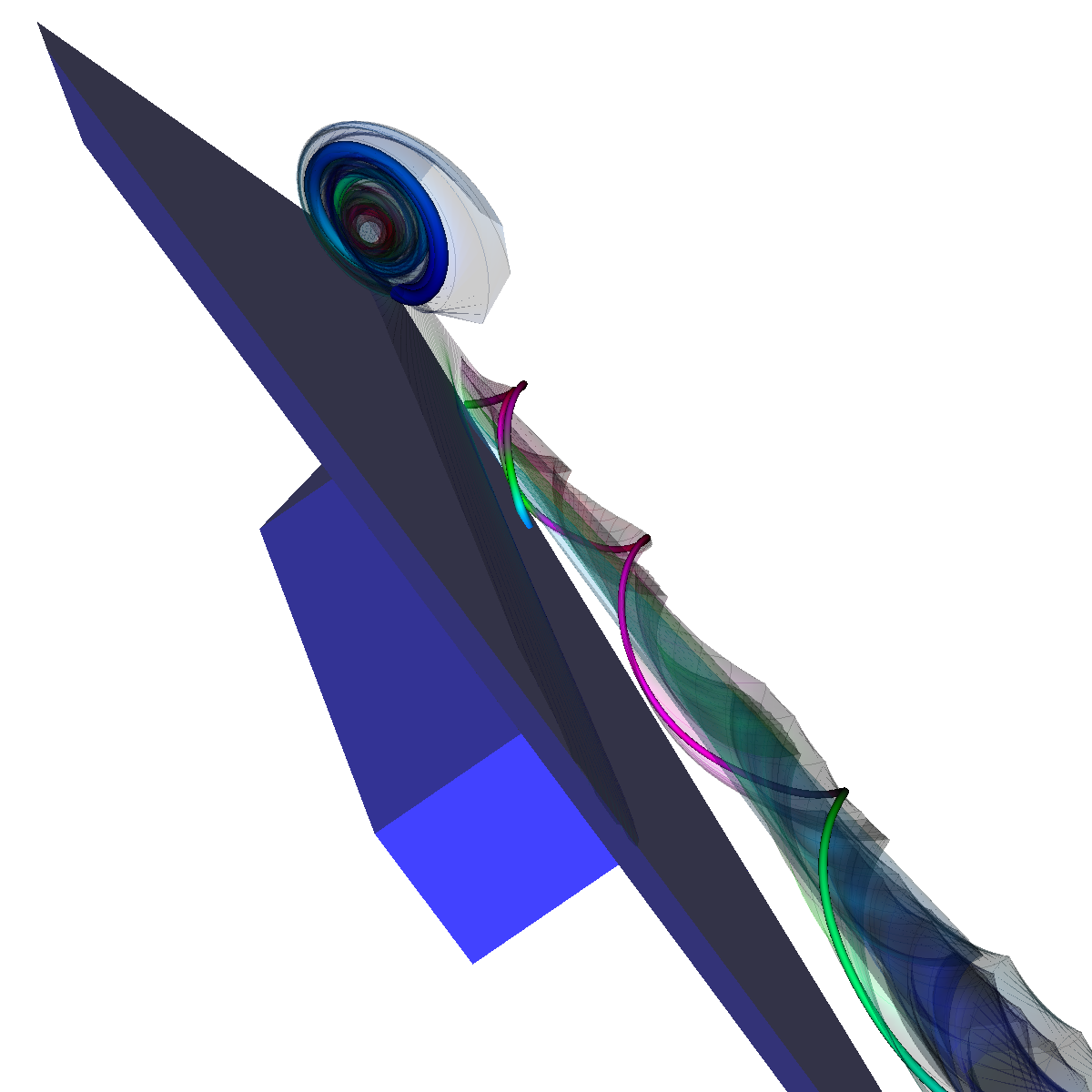 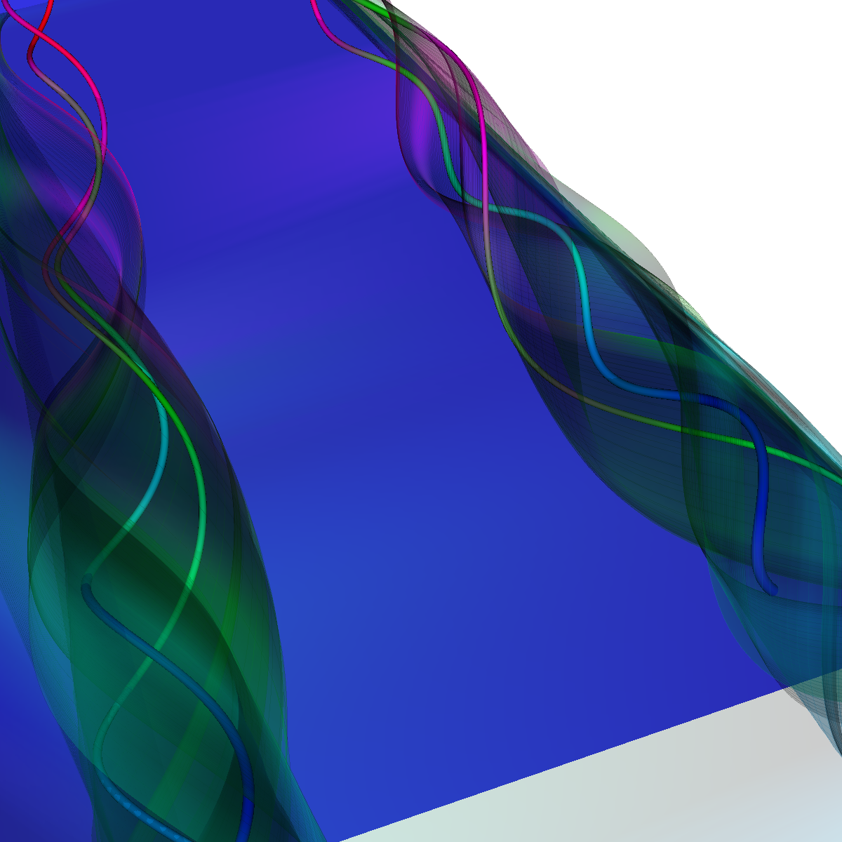 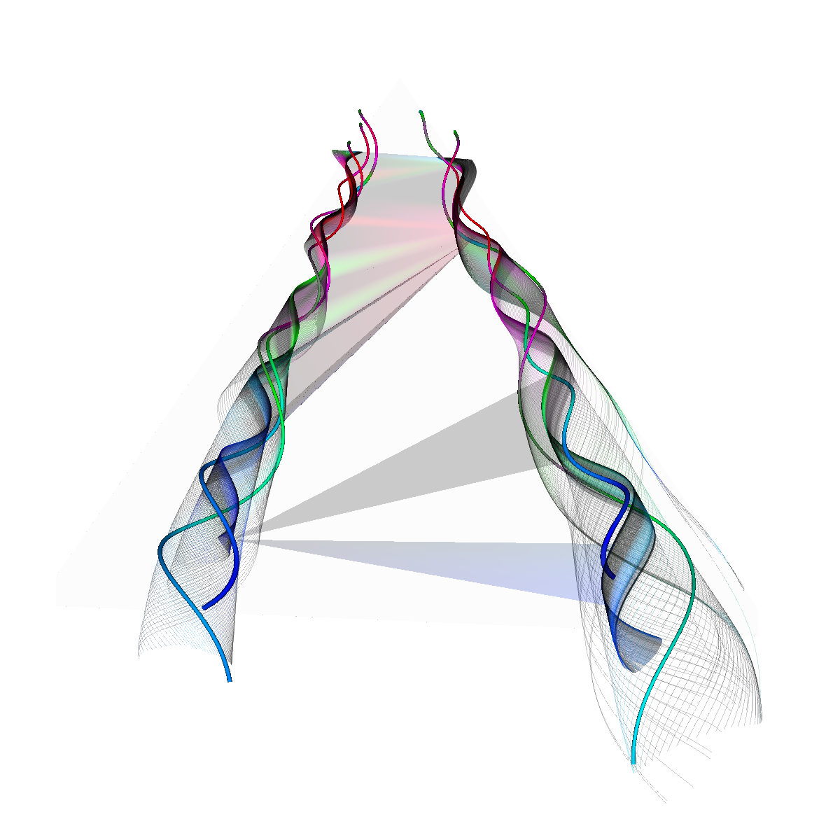 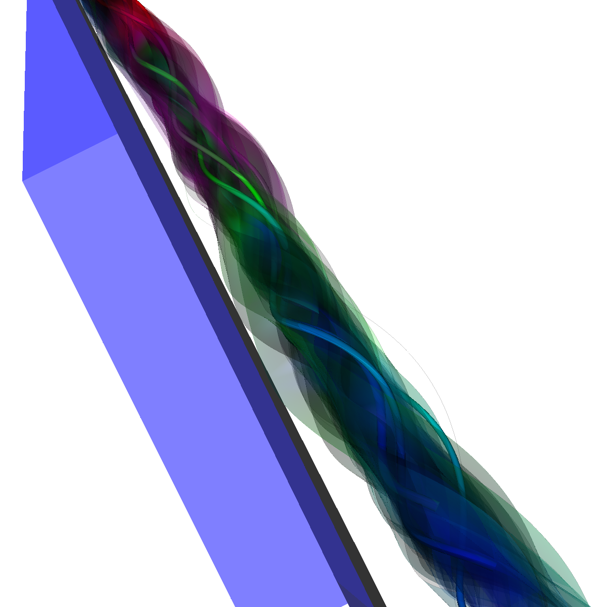 |
Part 6.2.1: Boundary Surface with Inner Surfaces We visualize the recirculation bubble by first choosing an appropriate line at location (30,120,0) to (30,-120,0) and applying stream surfaces (alpha=0.15) and streamlines. We include stream tubes as well as the wing geometry for context. We use a long line in order capture the flow along the boundaries (green surface) in an attempt to extract features from the vortex breakdown along the boundary. 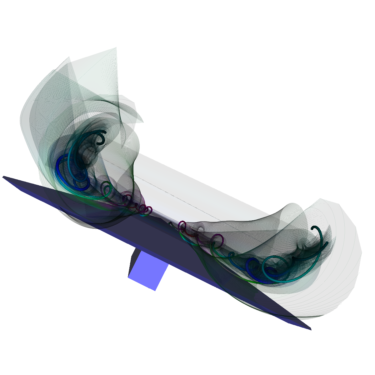 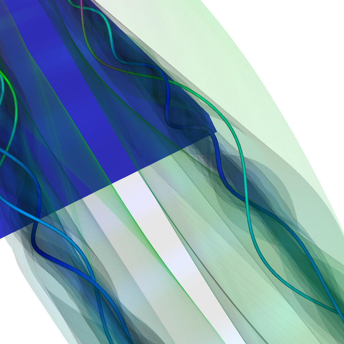 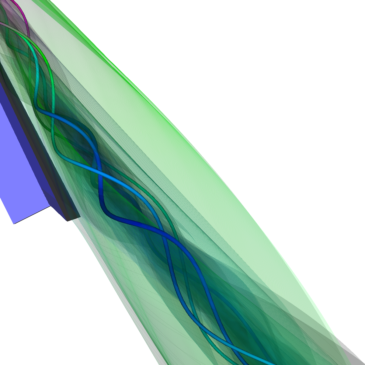 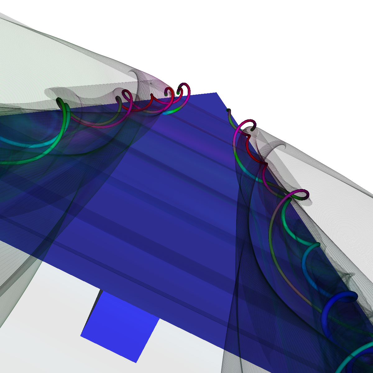 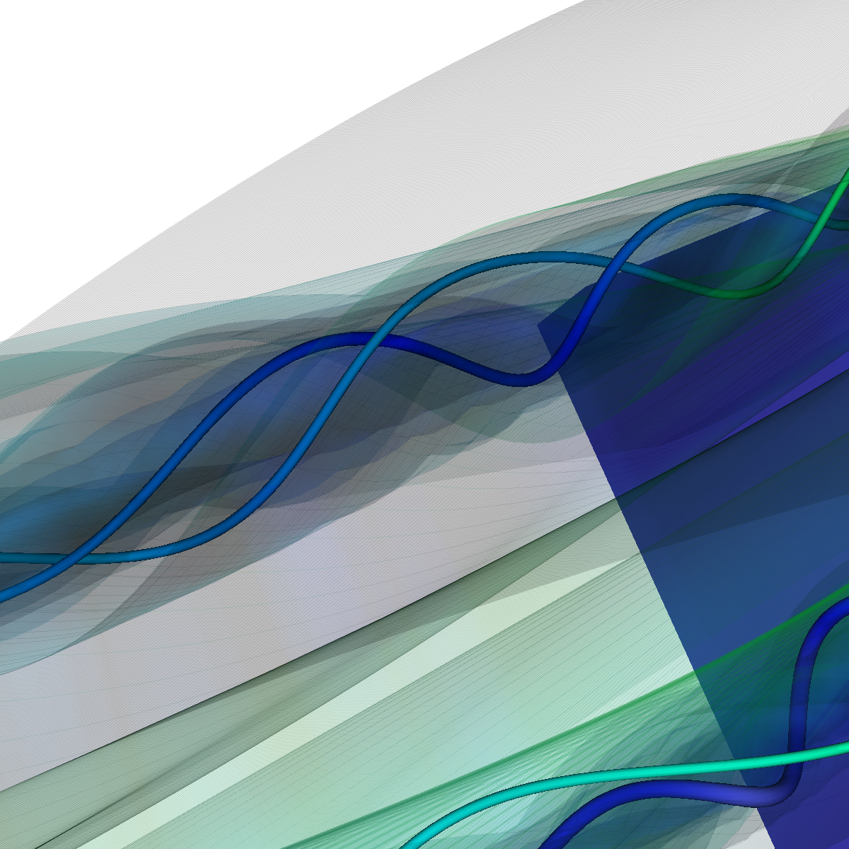 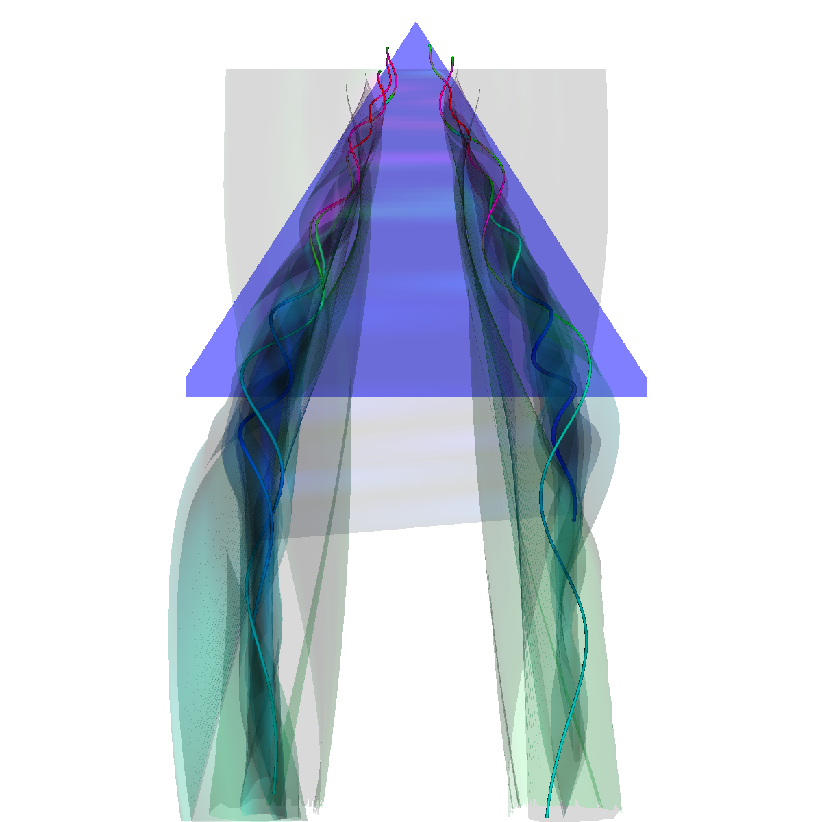 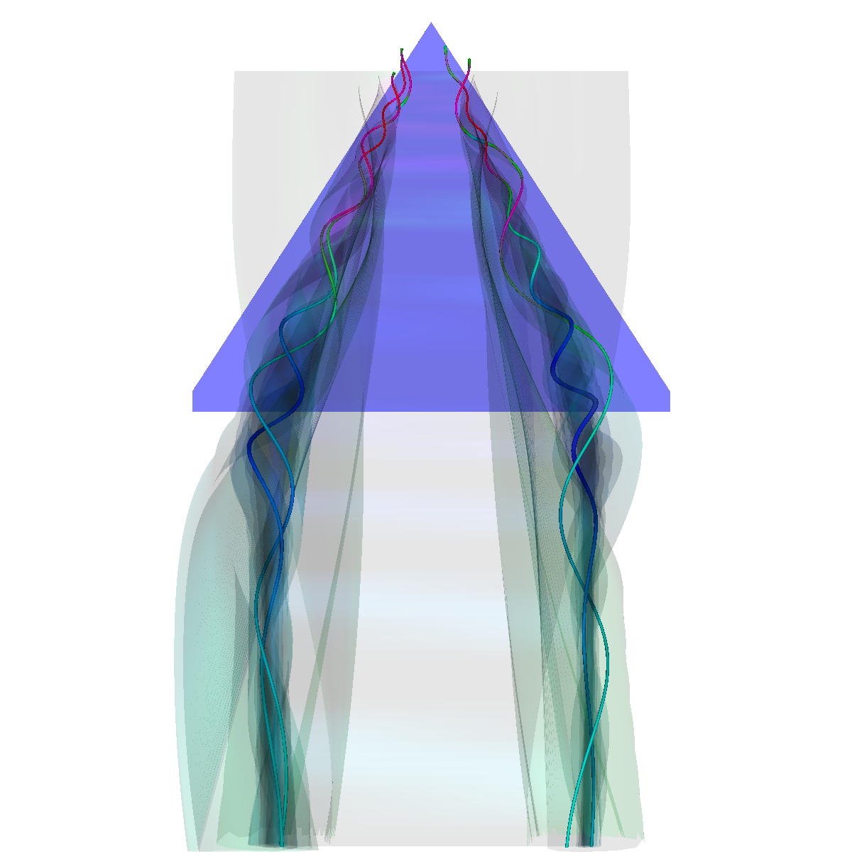 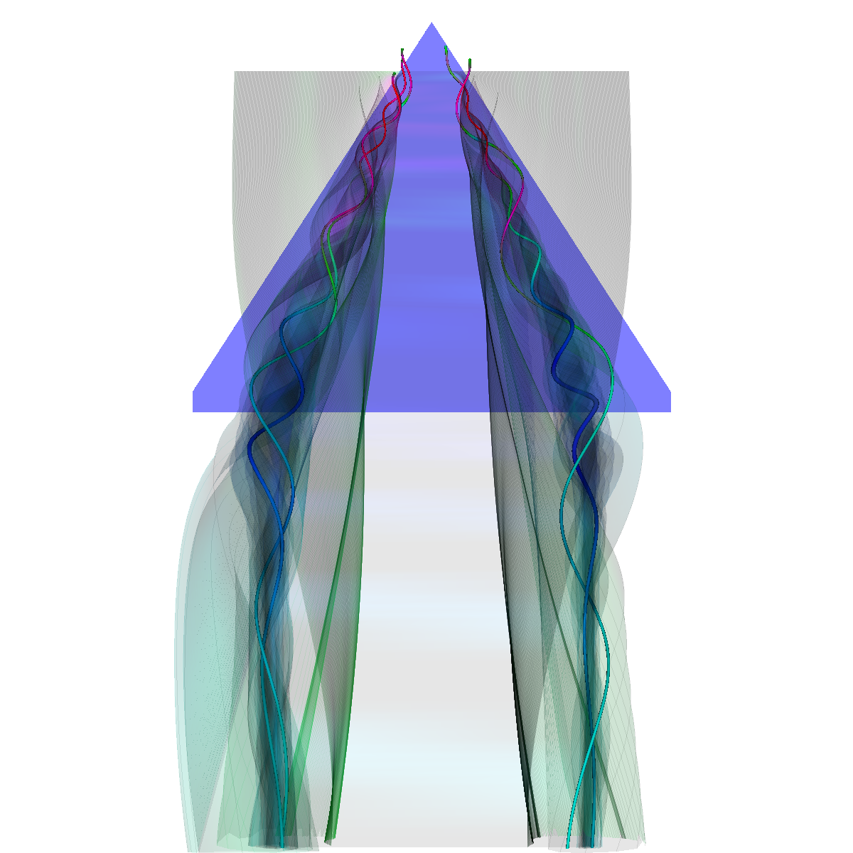 |
Part 6.2.2: Recirculation Bubble Seeded from (28,30,0) to (28,-30,0) We use stream surfaces and stream lines. We include a few stream tubes and the wing geometry for context. We also adjusted settings for the stream surface. The vortex breakdown features are captured by adjusting integration, stitching, and other arbitrary parameters such as opaqueness. We found that drastically different stream surfaces are generated by the stitching mode (resampling or walking points). 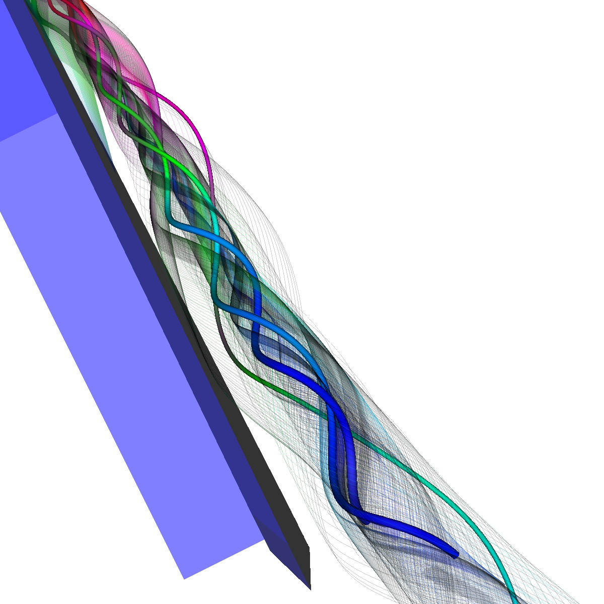 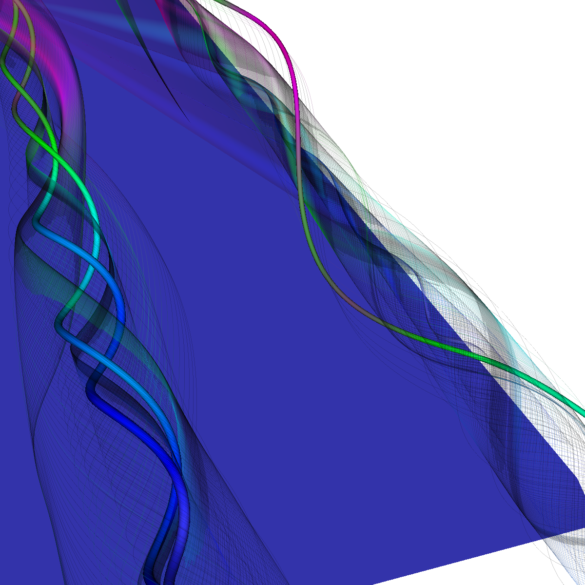 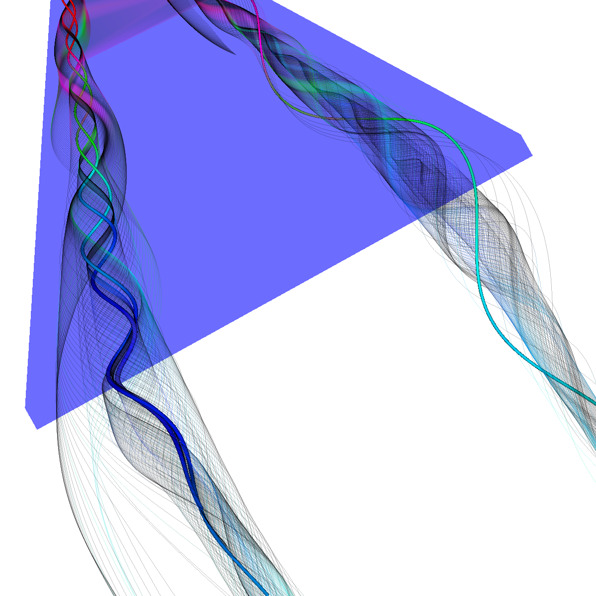 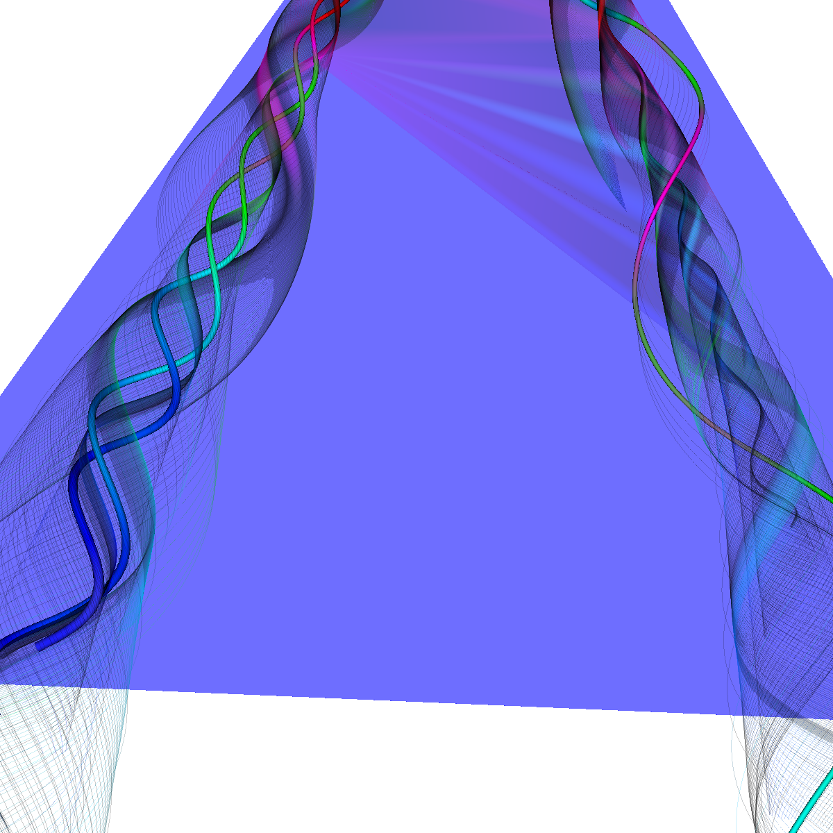 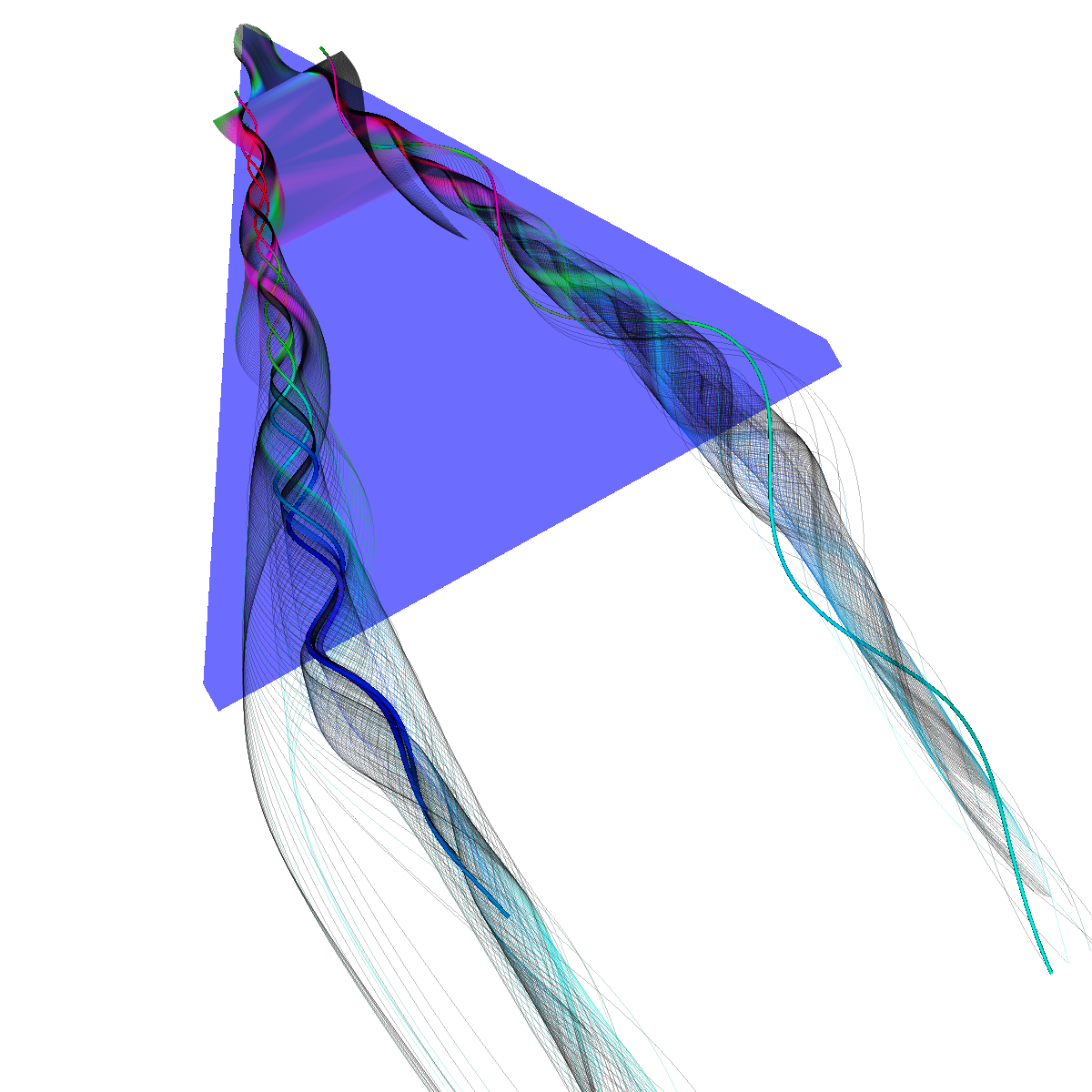 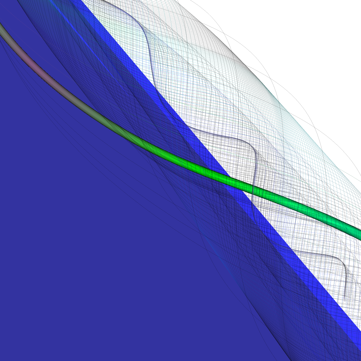 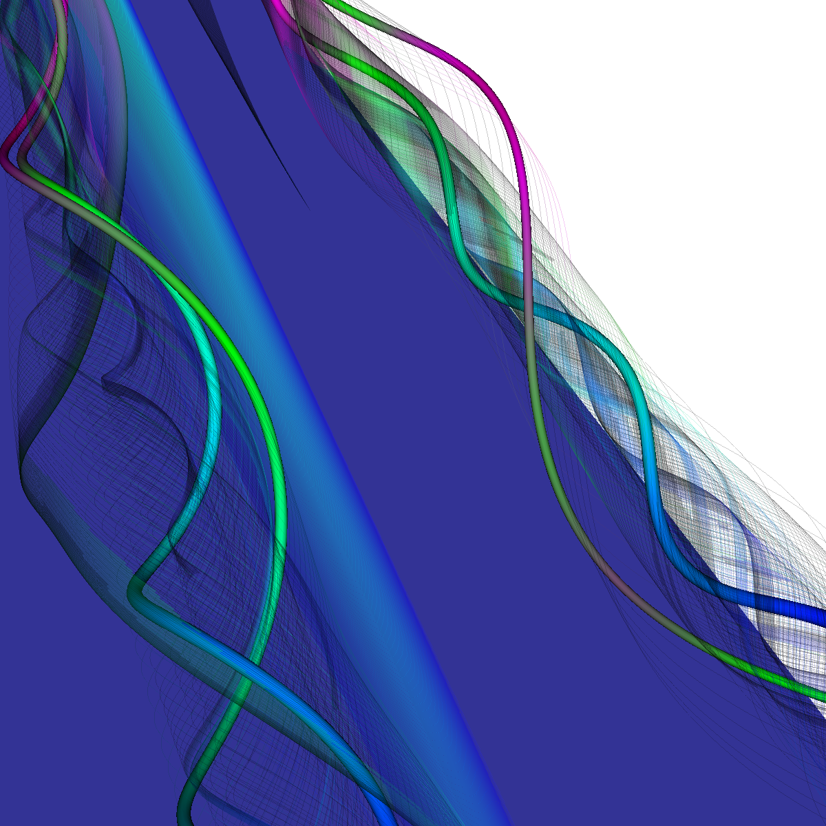 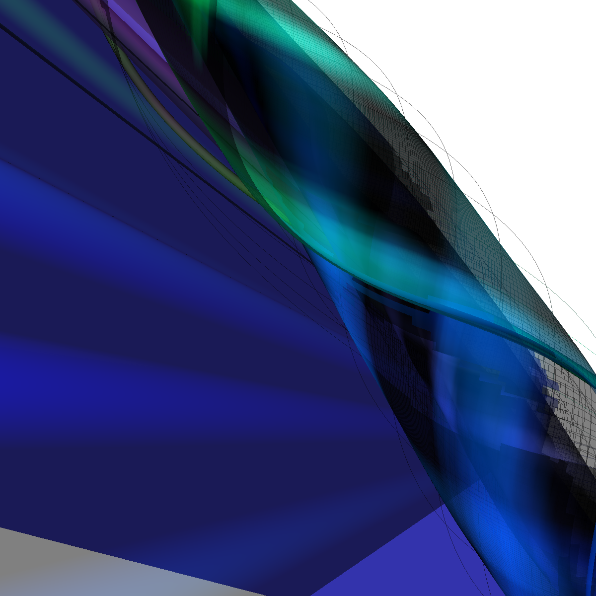 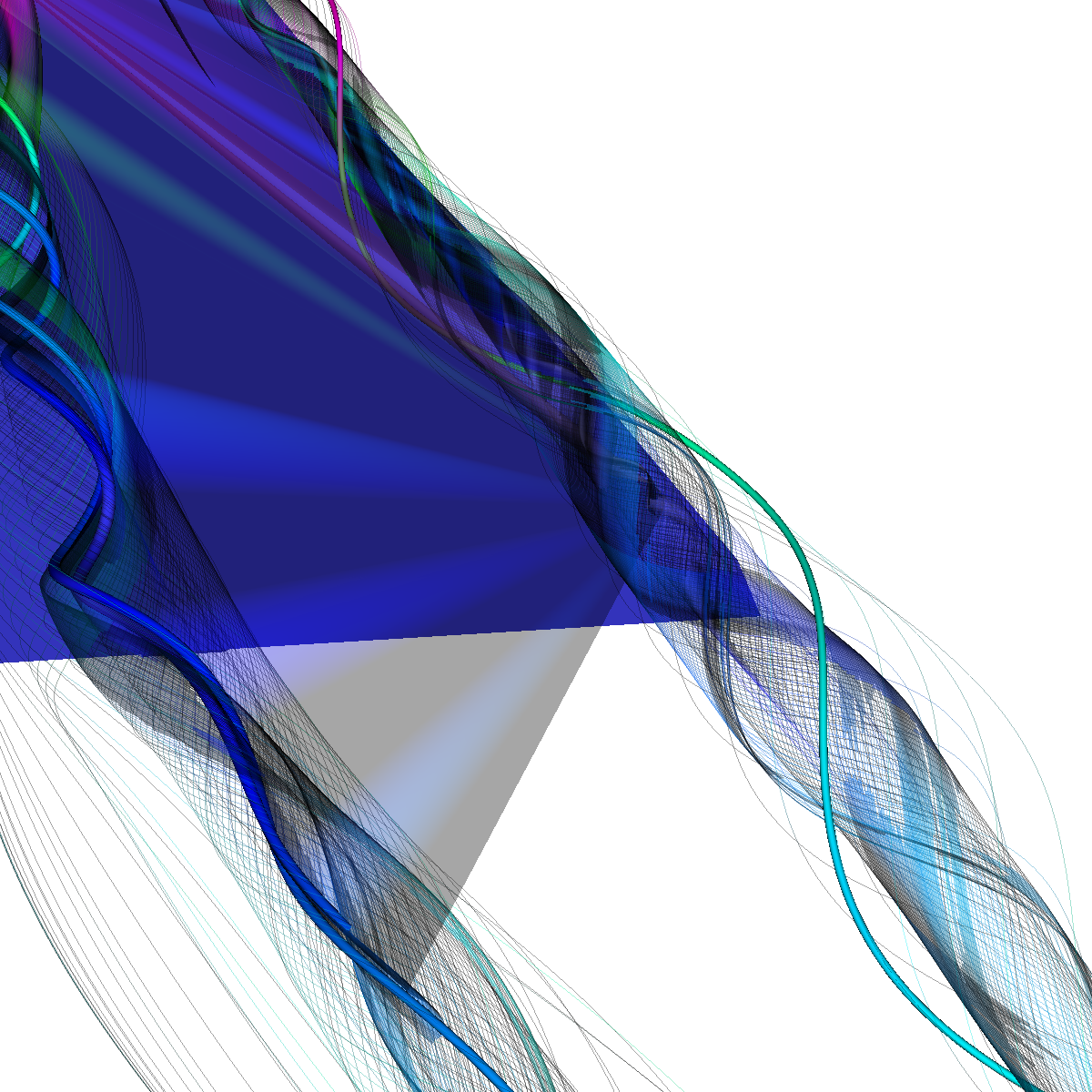 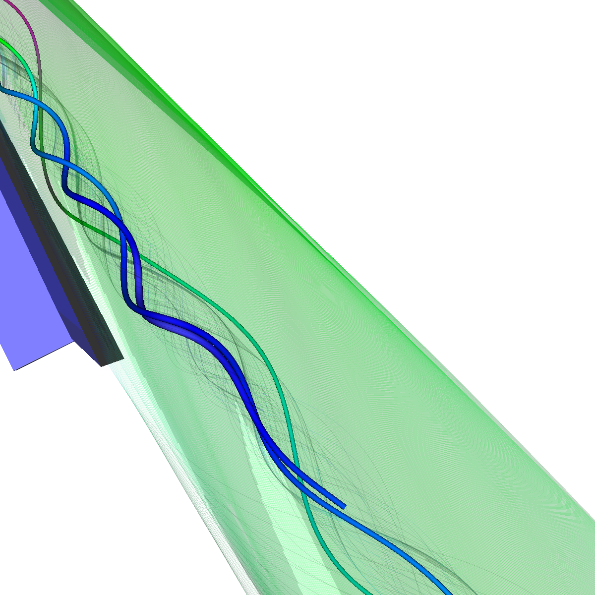 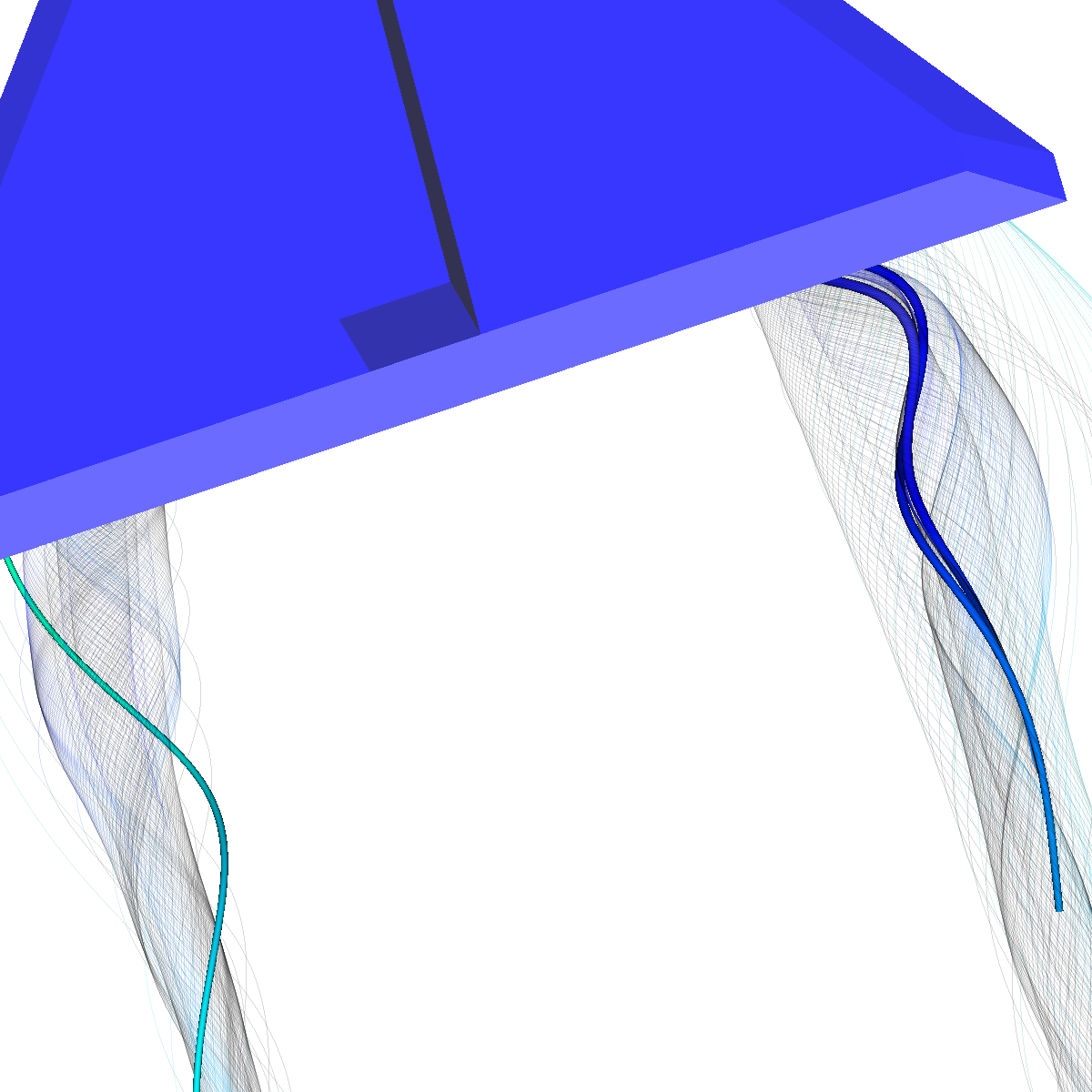 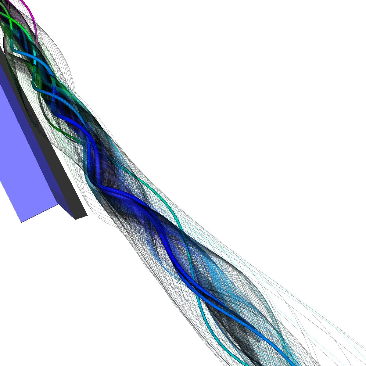 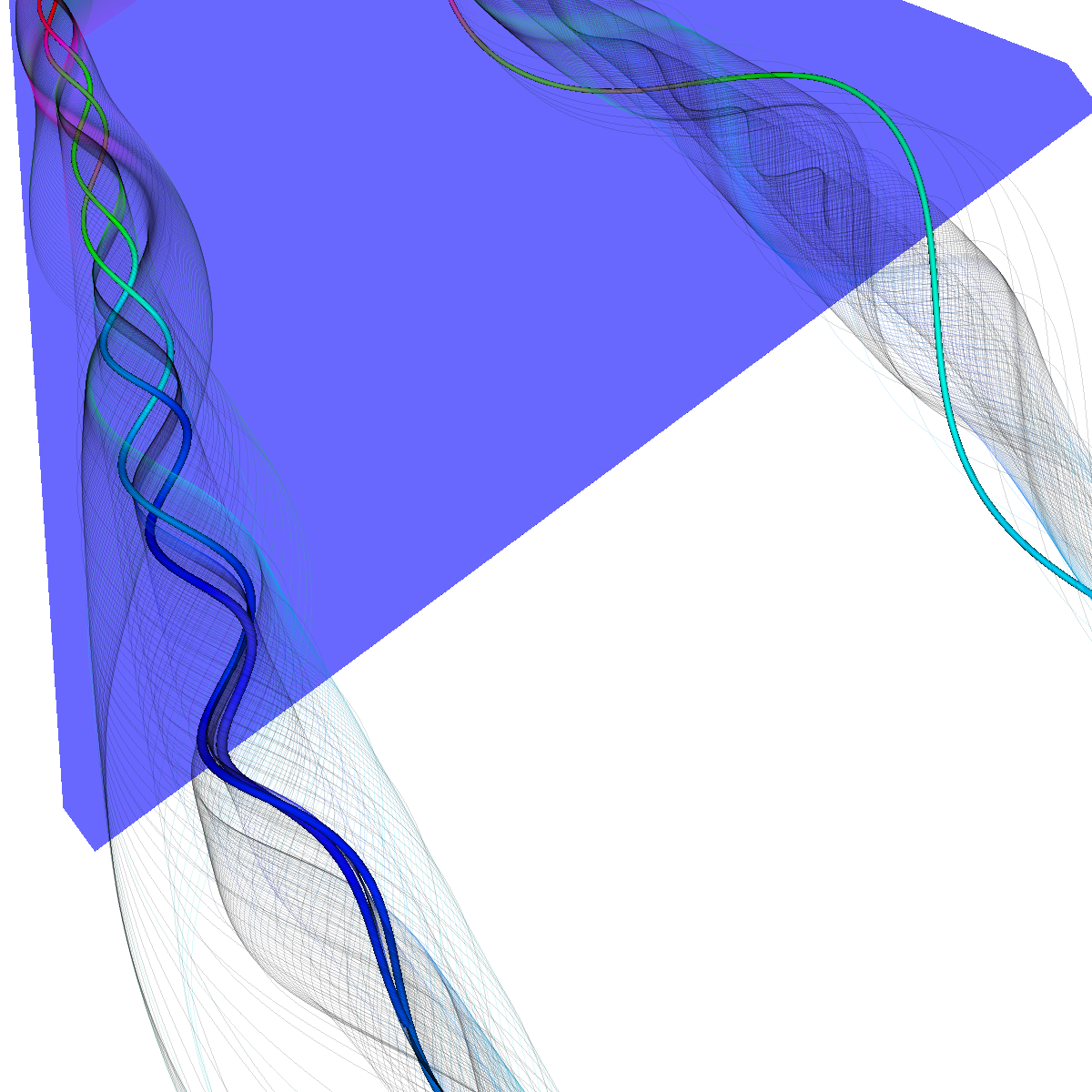 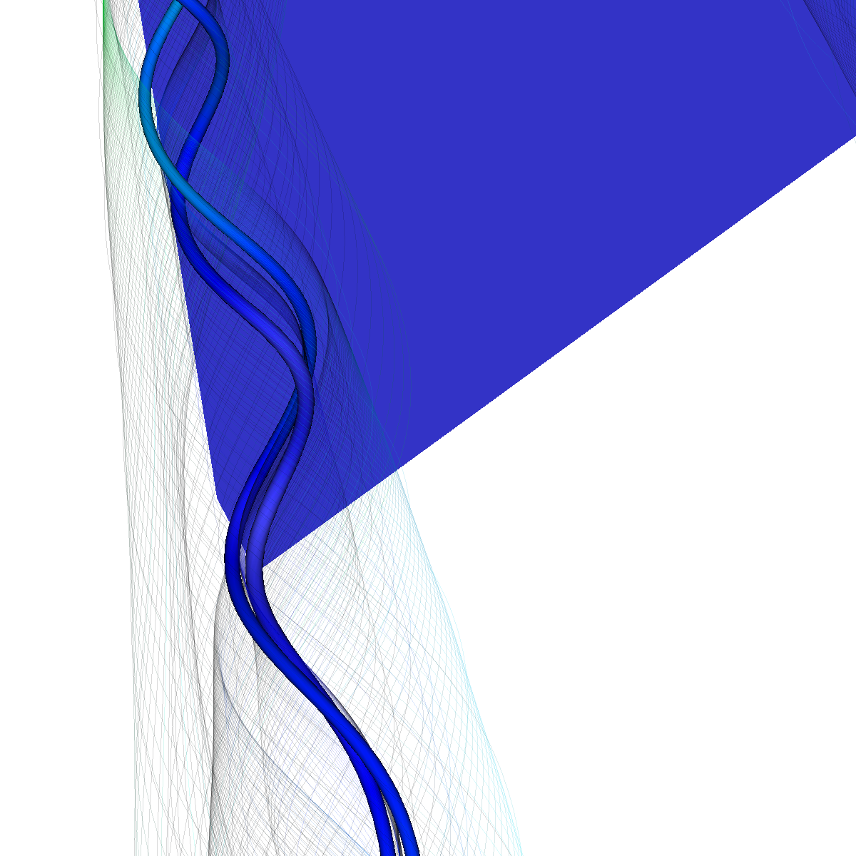 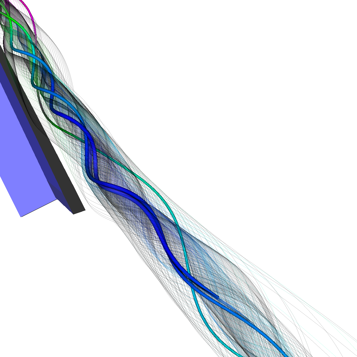 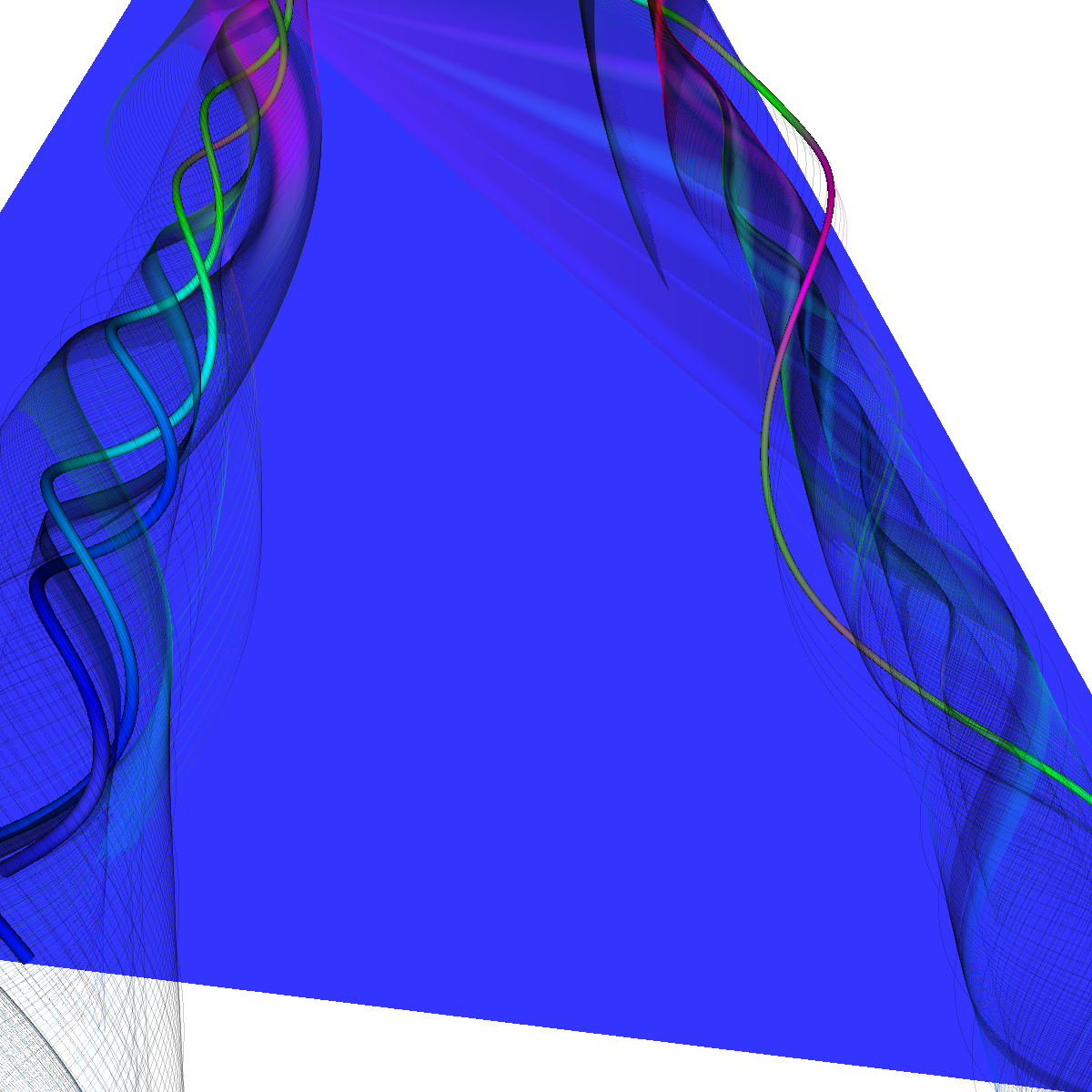 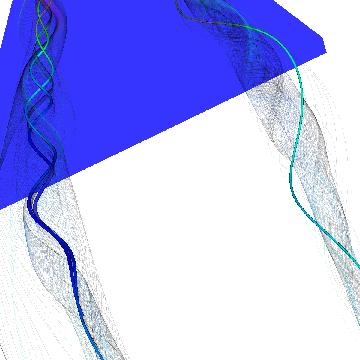 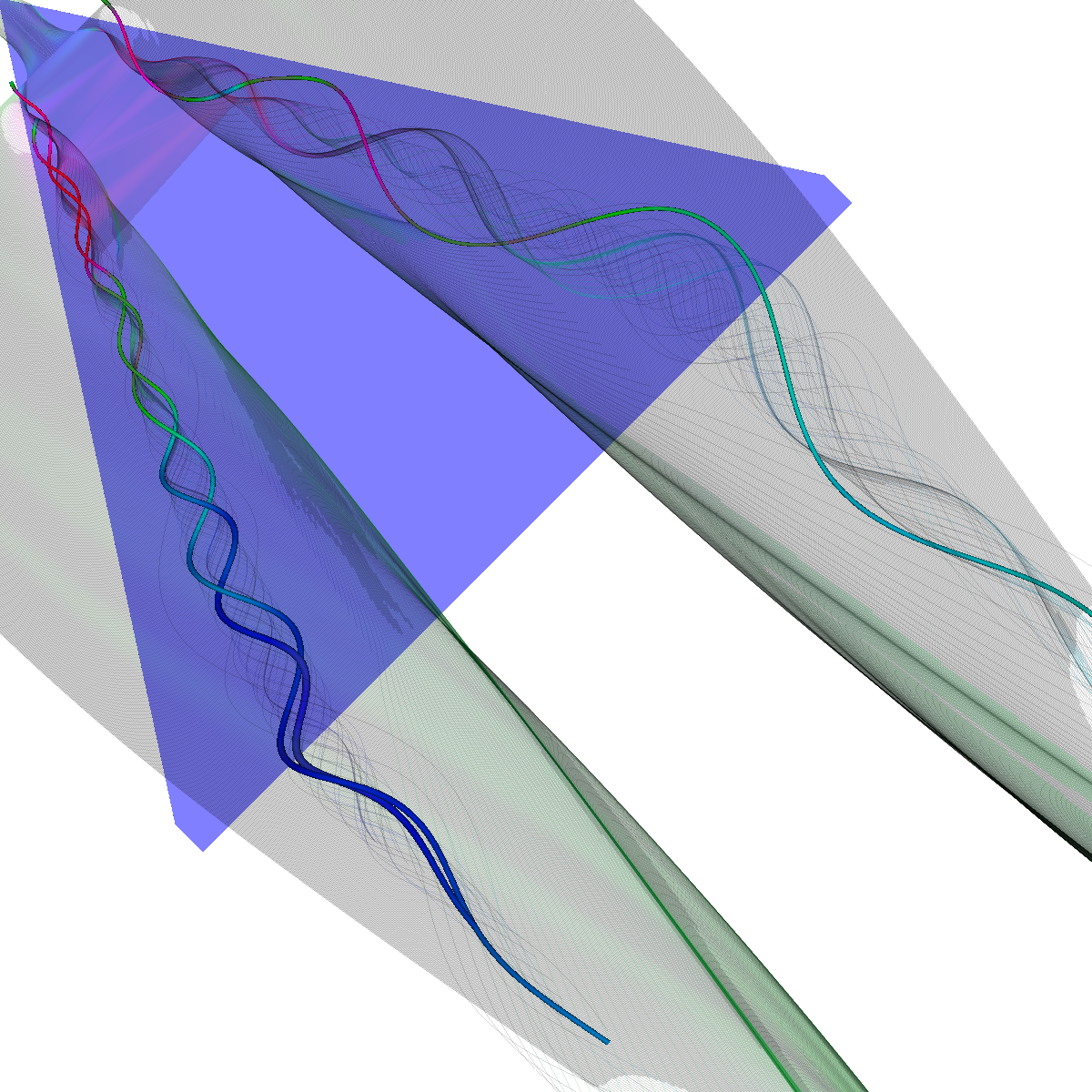 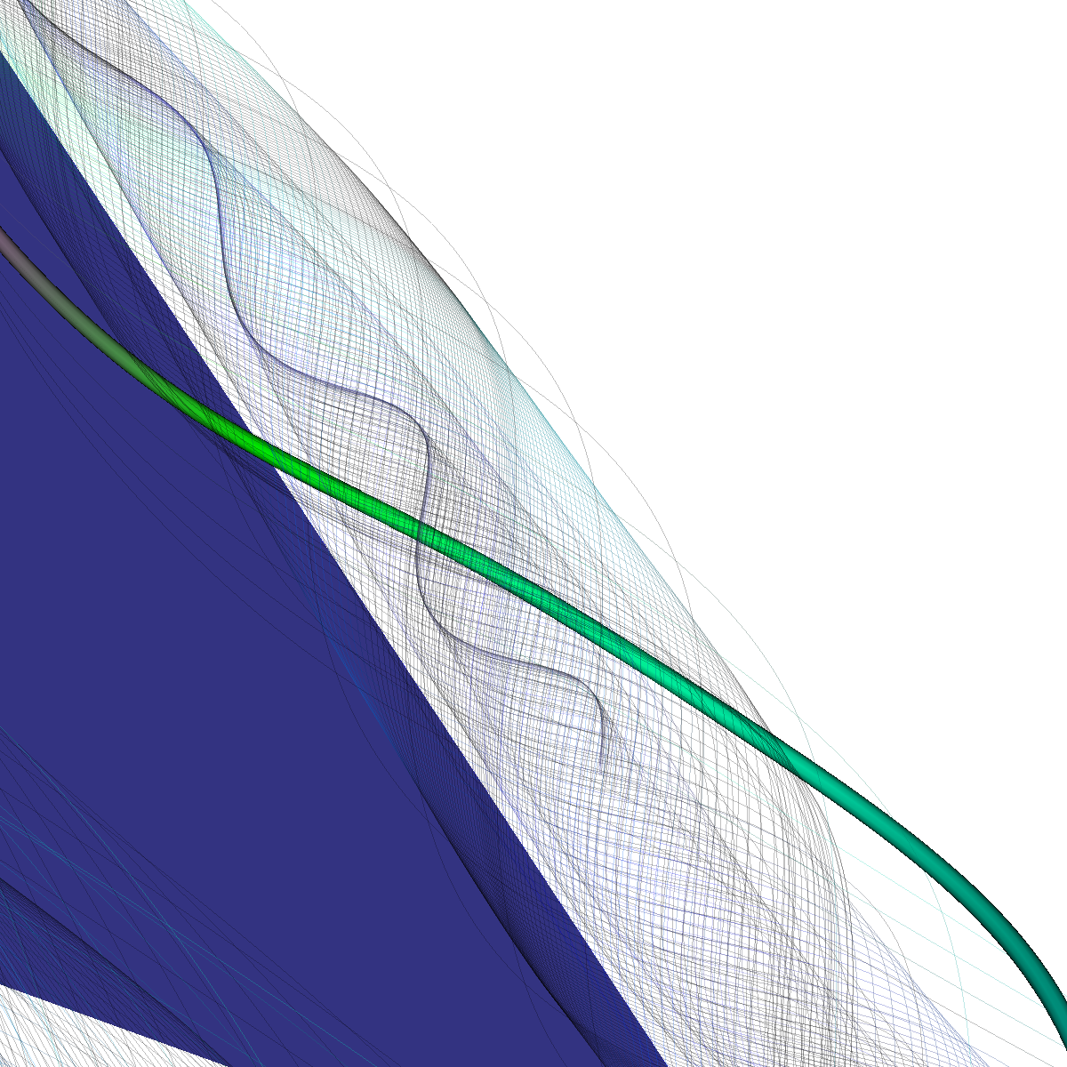 |
Part 6.2.3: Seeding stream surfaces This time we defined the stream surface by using the two points (40,20,0) to (40,-20,0) as centers and randomly sampling seed locations up to a radius of 10-20 from the center points. We then cleaned the streamlines from the forward integration and stitched them together to generate the stream surface (alpha=0.15). We include stream tubes as well as the wing geometry for context. We chose to use this type of seeding in an attempt to highlight features from the inner stream surfaces. This seeding method forms more tightly knit stream surfaces. |
Part 6.2.4: Recirculation Bubble Seeded along the line (50,40,5) to (50,-40,5) We apply stream surfaces seeded along the line defined by the points (50,40,5) to (50,-40,5). We apply a range of techniques in order to extract the most significant features (as previously discussed). 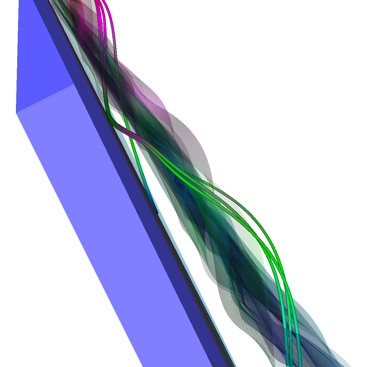 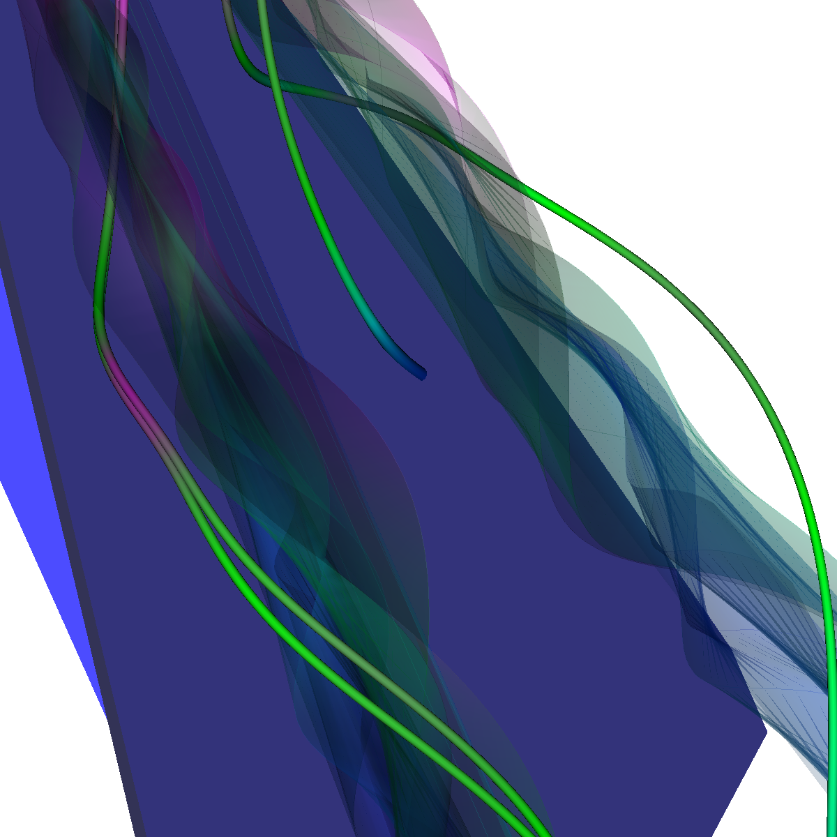 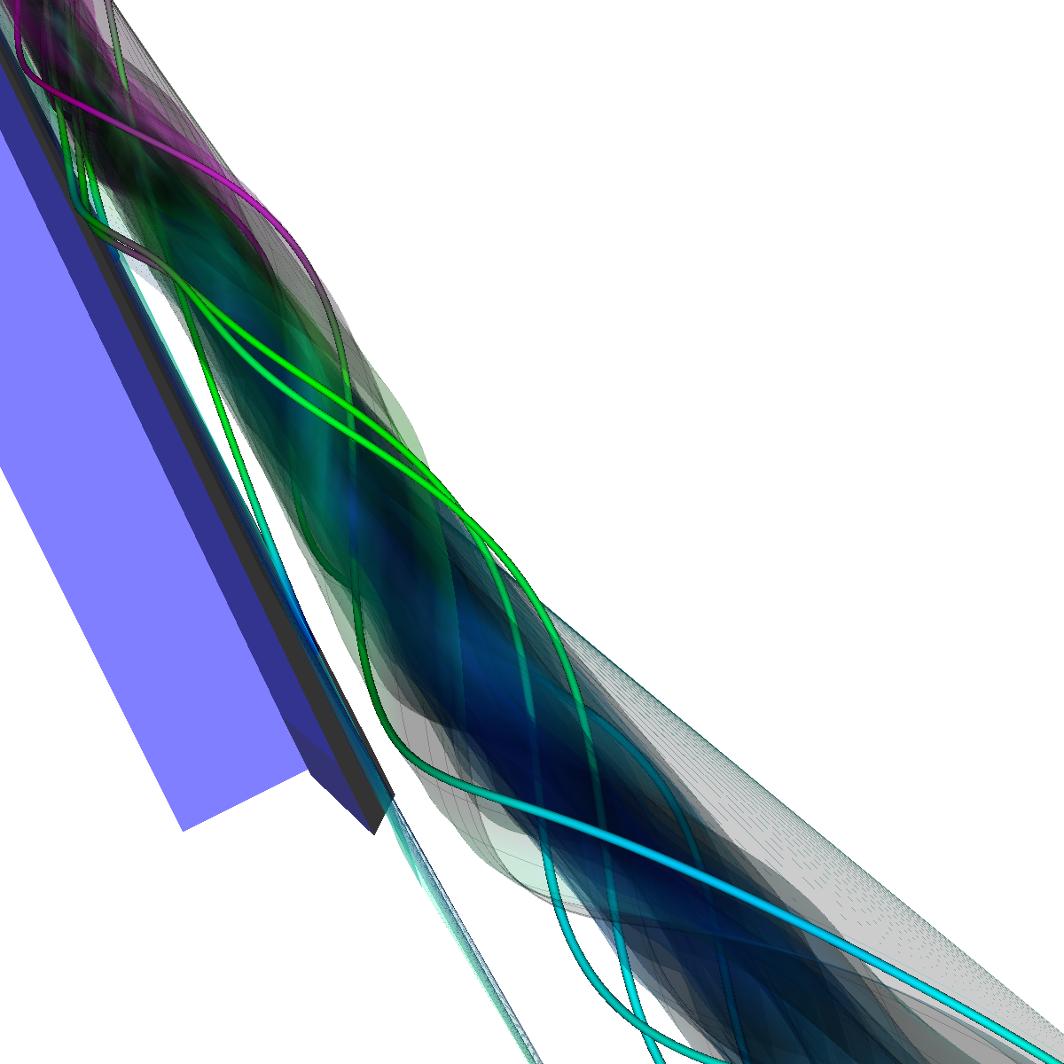 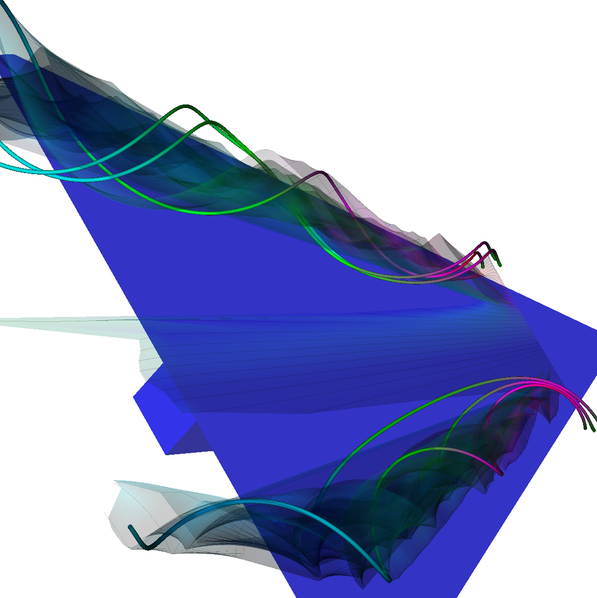 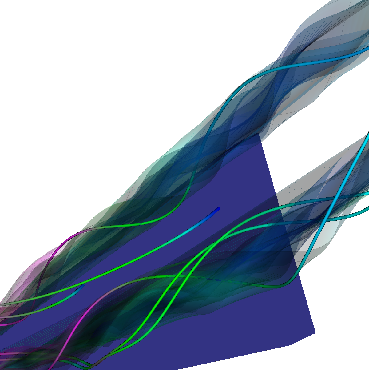 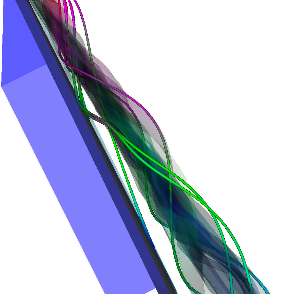 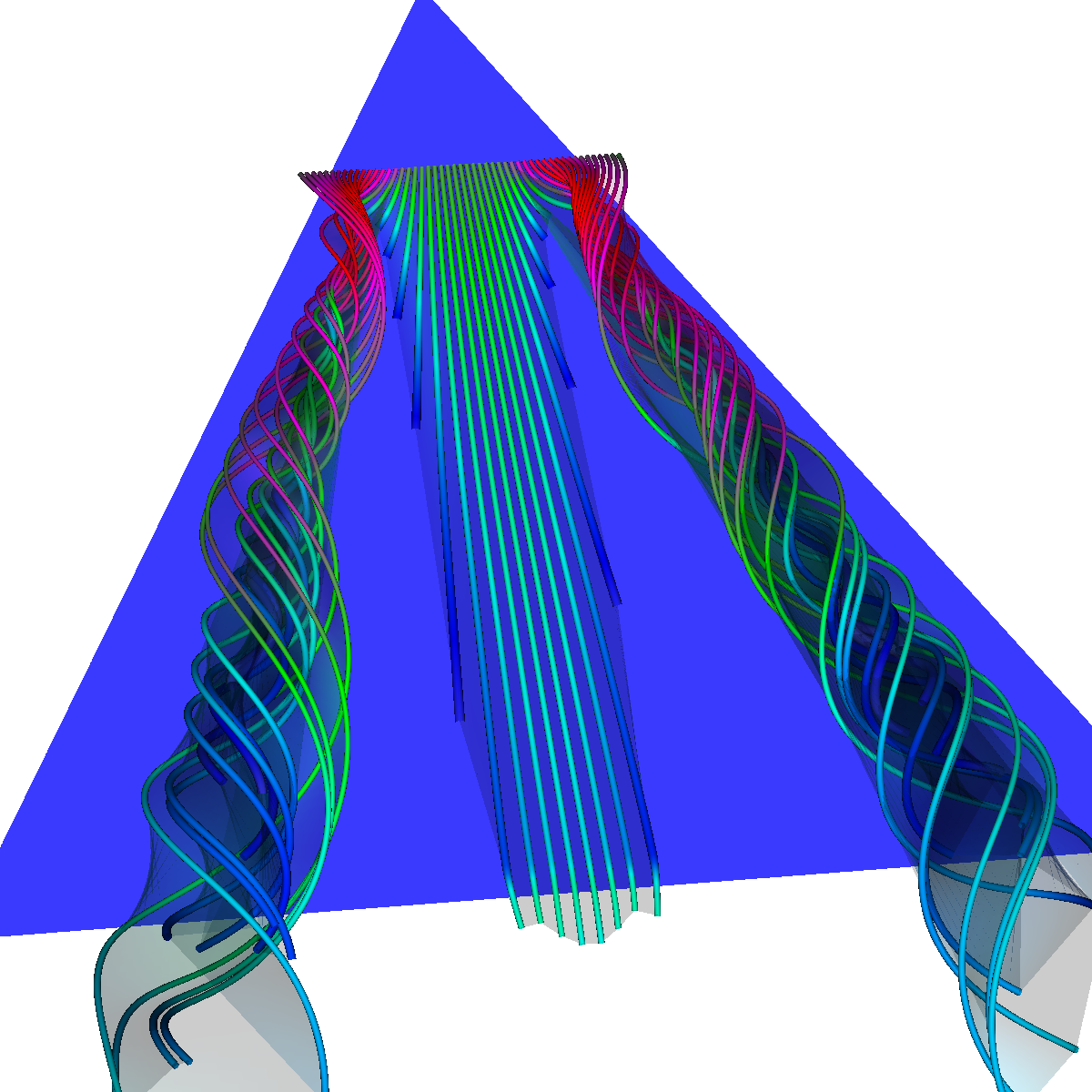 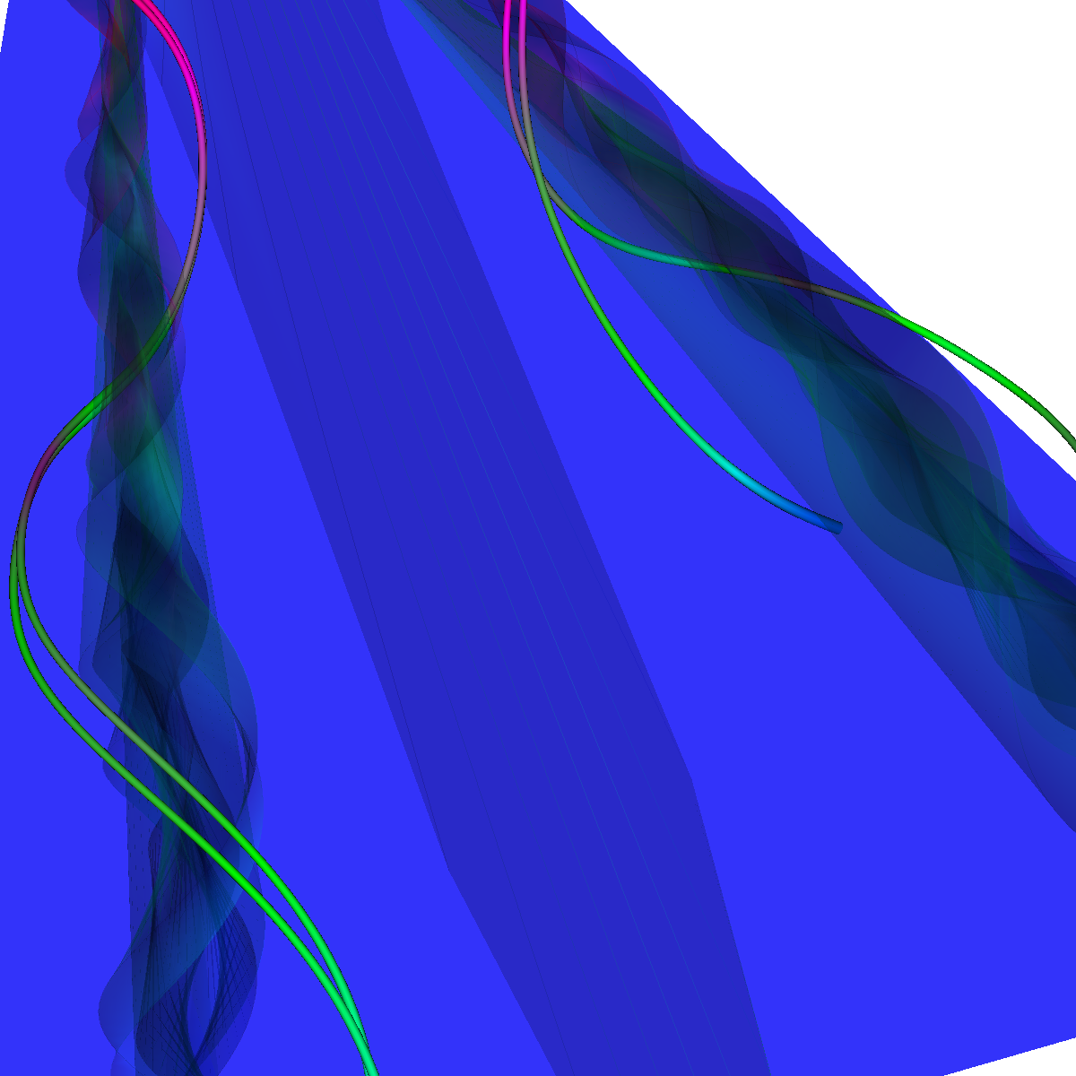 |
Part 6.2.5: Vortex breakdown We visualize the vortex breakdown by first randomly sampling from the line (70,50,0) to (70,-50,0) and applying stream surfaces (alpha=0.15) and stream tubes. We include stream tubes as well as the wing geometry for context. 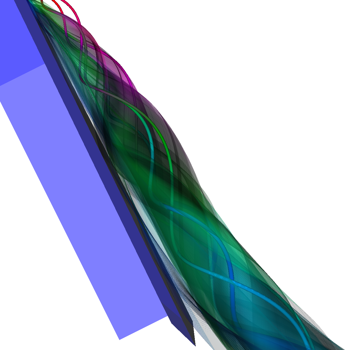 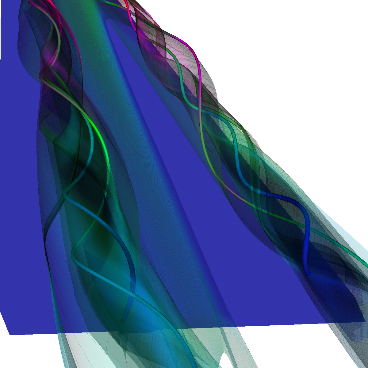 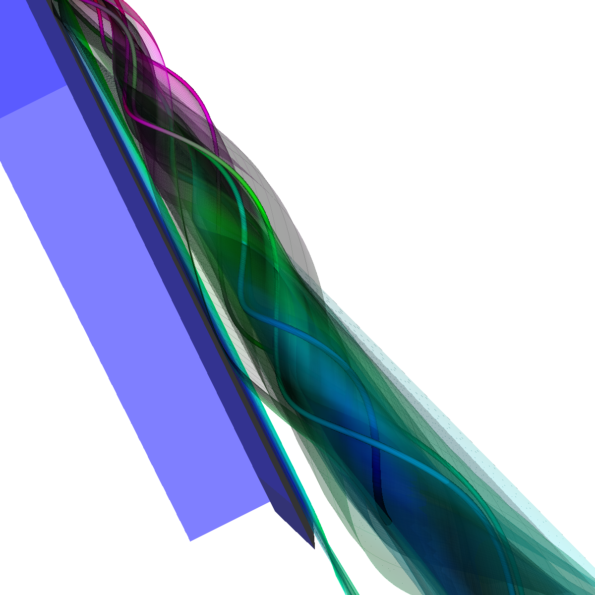 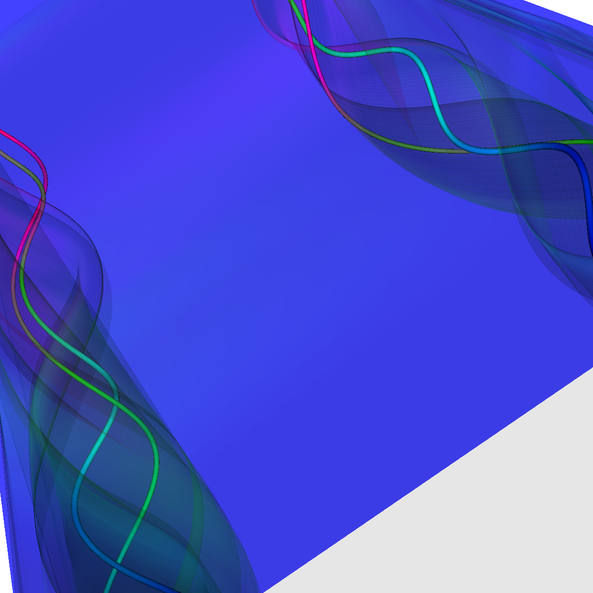 |
Part 6.2.6: Other integration schemes We then apply other integration schemes such as Runge-Kutta45 and vary the number of streamlines used to generate the stream surfaces below. We also apply a cleaner to remove noise from the integration. 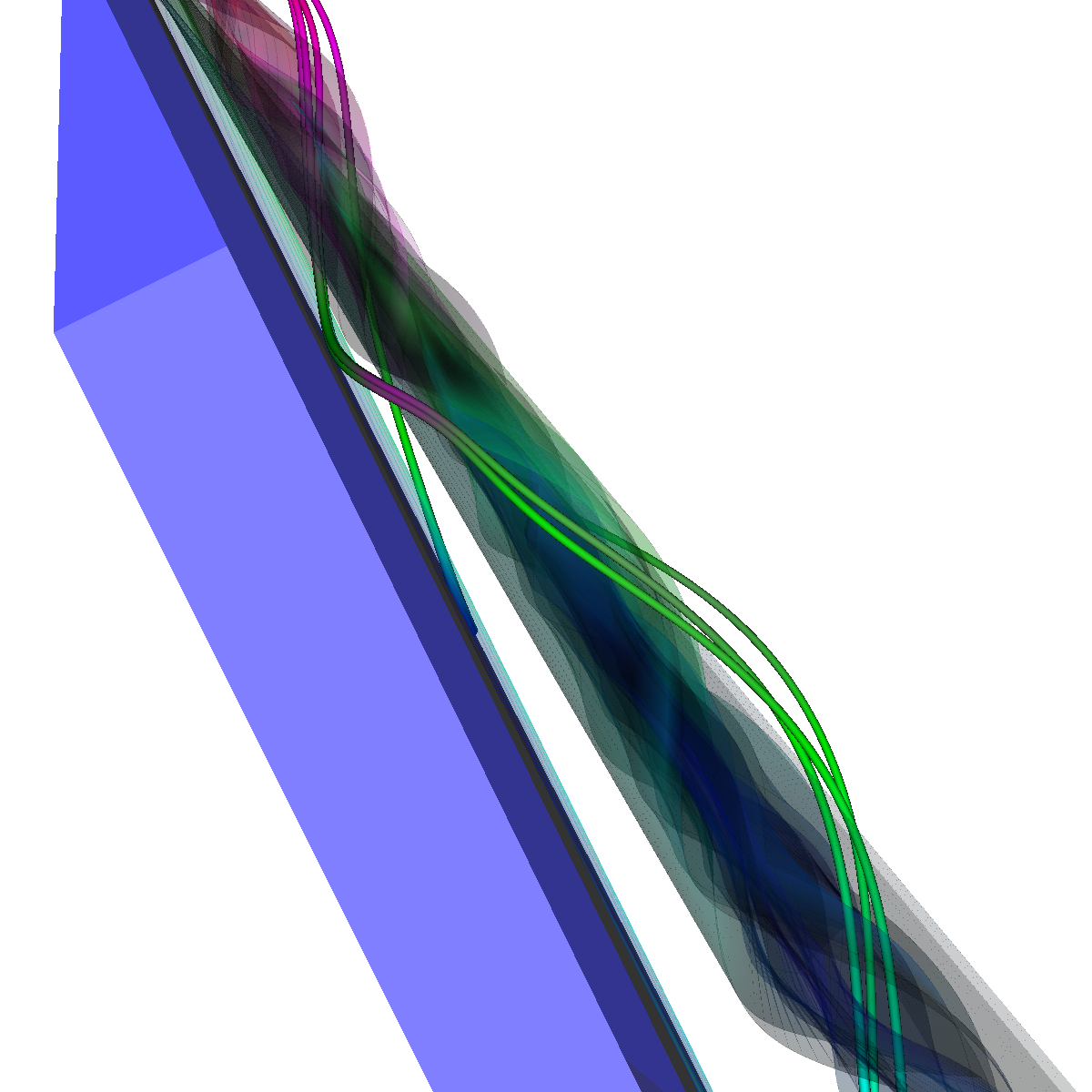 |
Part 6.2.7: Other attempts at visualizing the recirculation bubble We created a line at (40,30,0) and (40,-30,0) and applied stream surfaces with a relatively small step size creating a somewhat smooth surface. This visualization is useful to extract the essence of the vortex breakdown without many details. 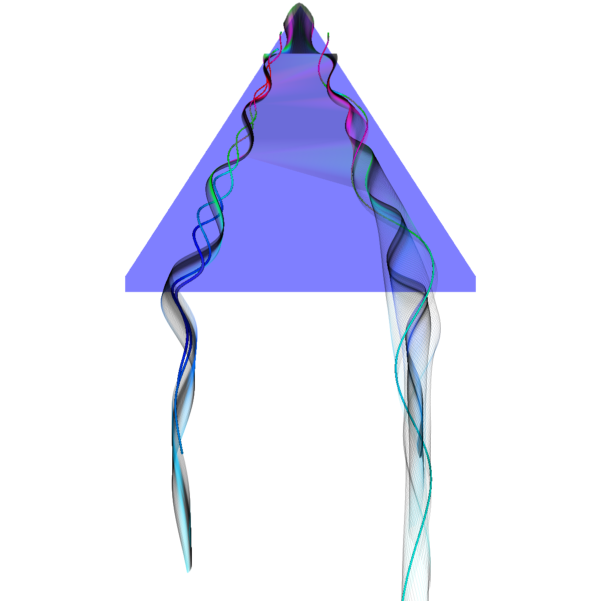 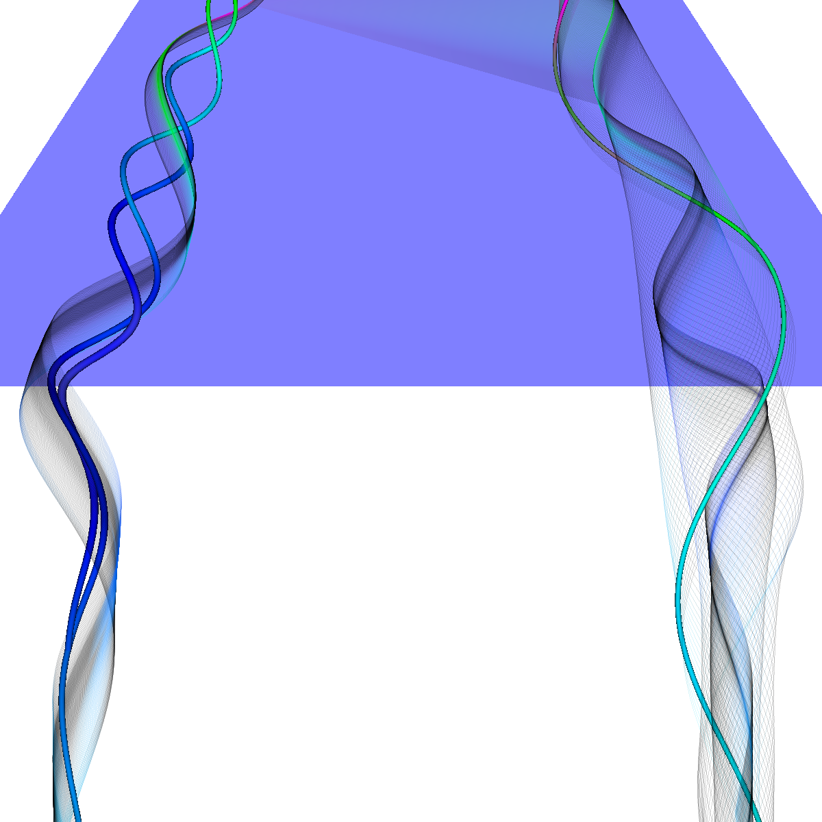 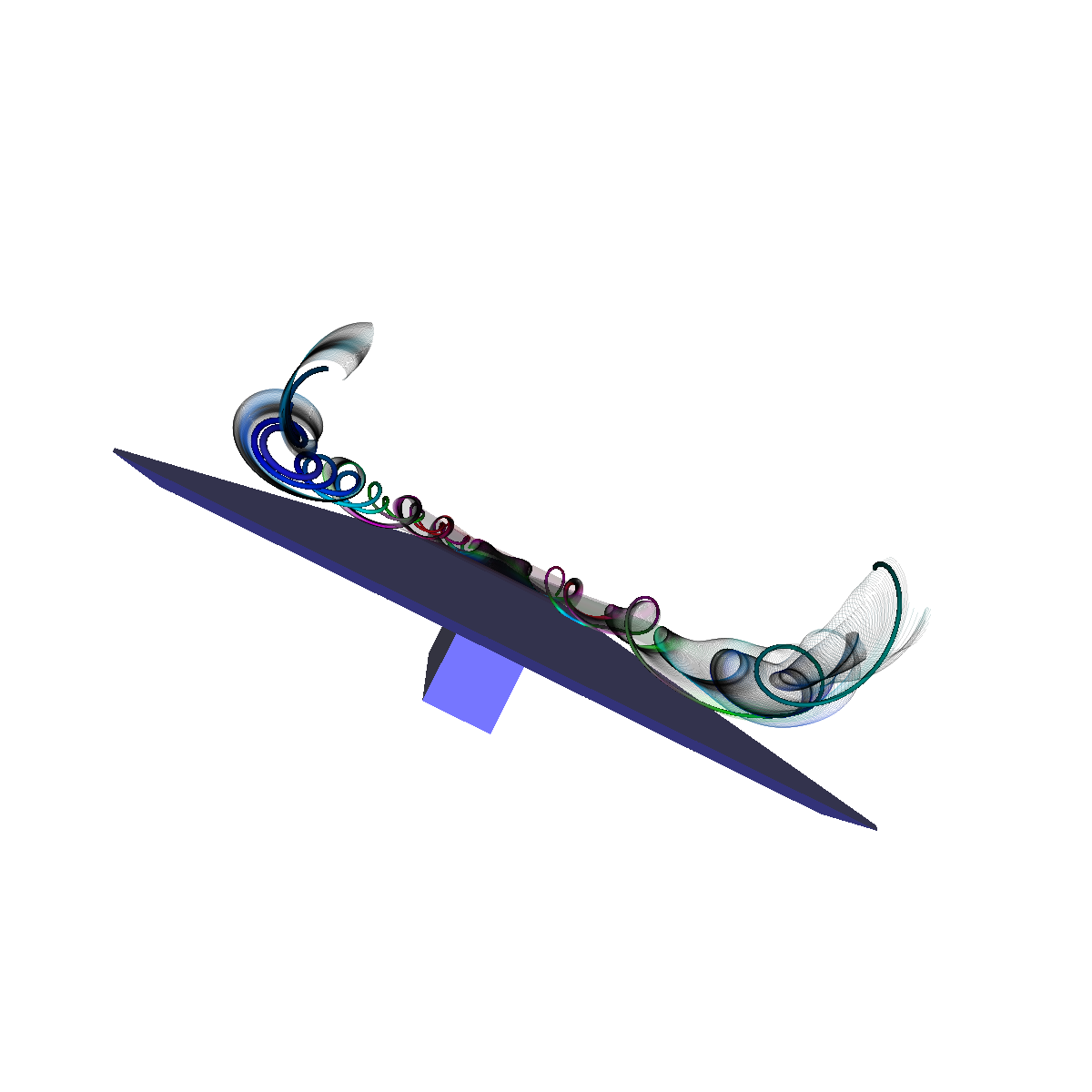 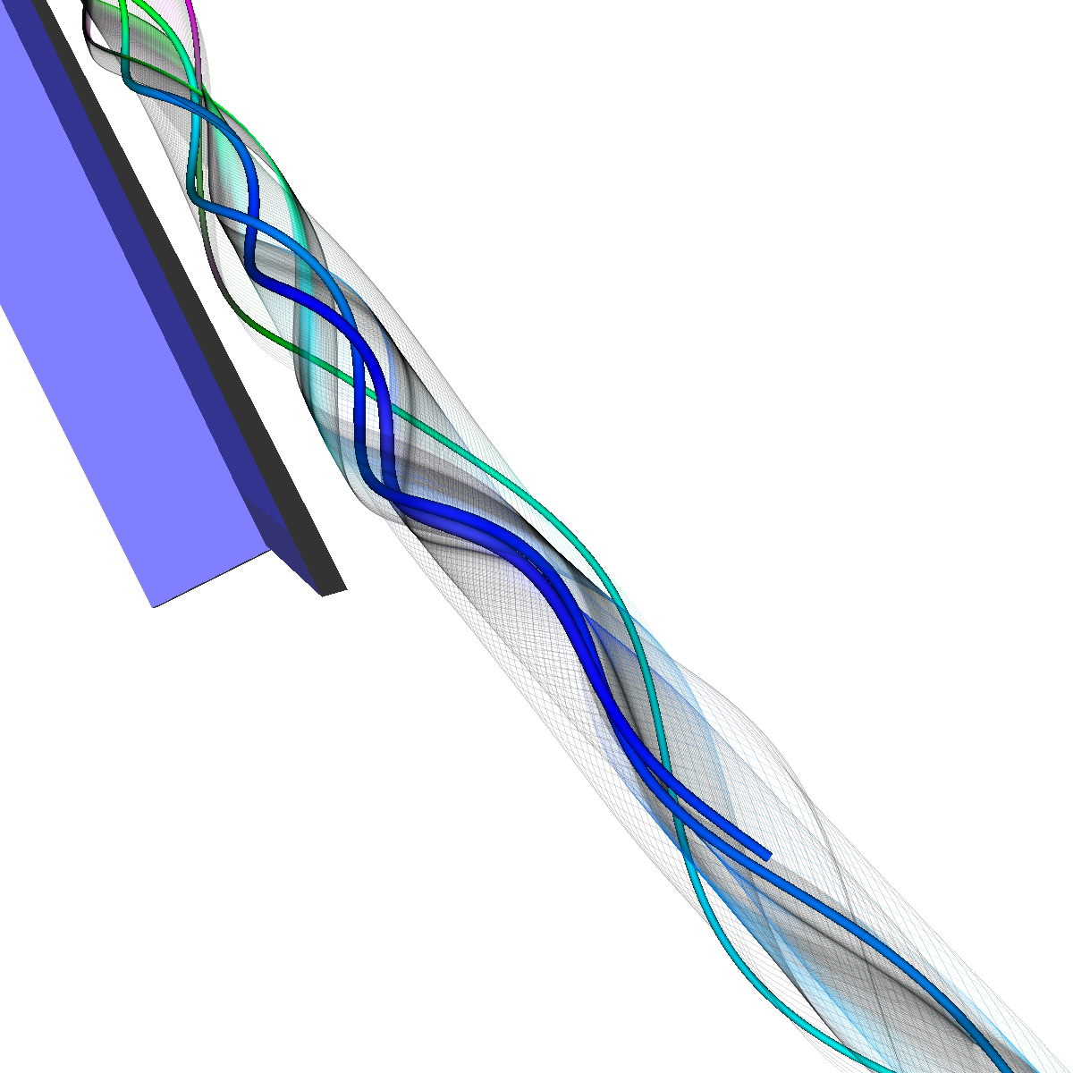 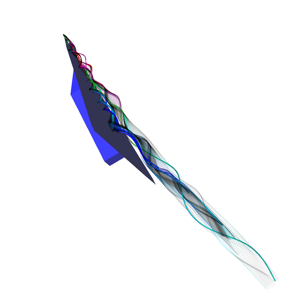 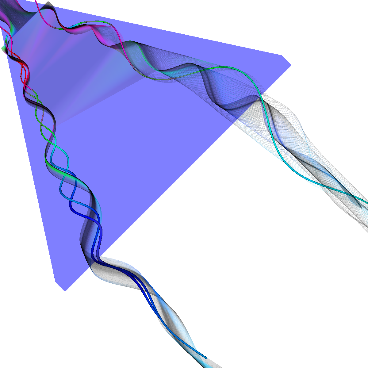 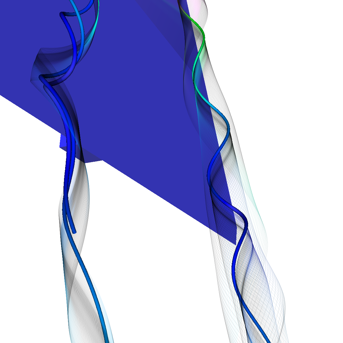 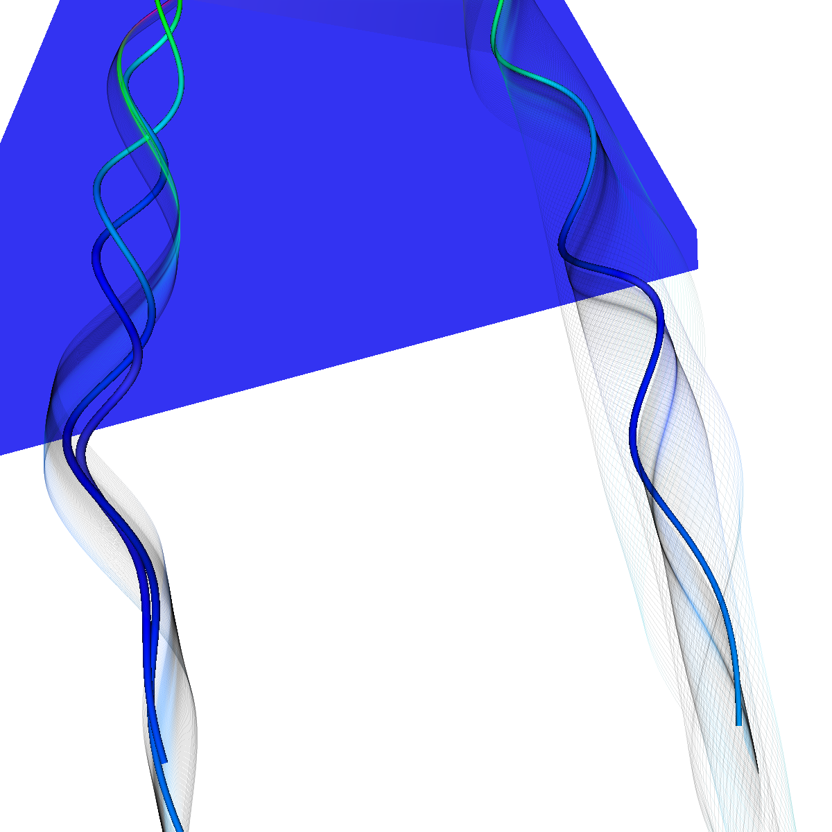 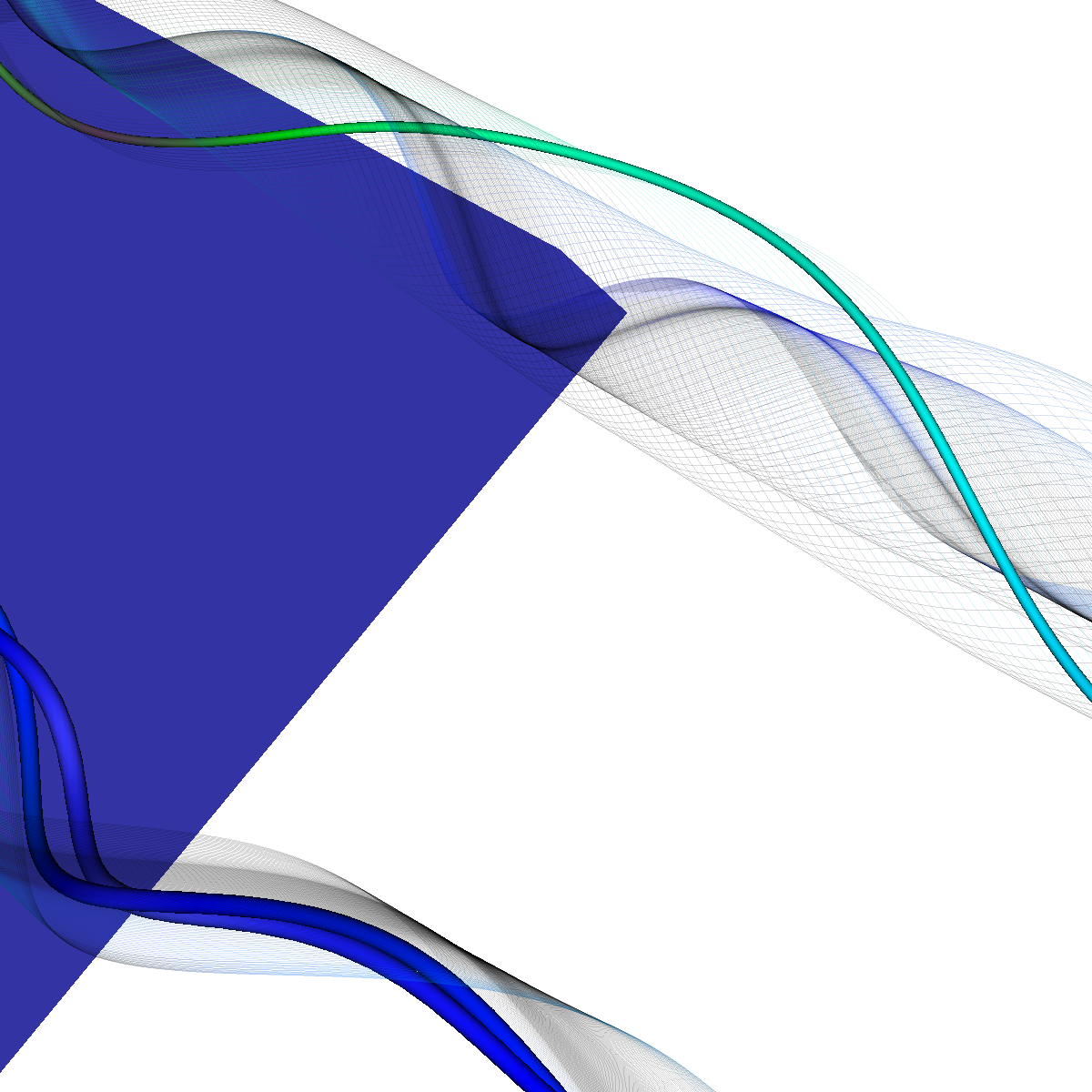 |
Part 6.2.8: Other attempts at visualizing the recirculation bubble We apply a variety of techniques in an attempt to extract some of the other hidden features. In essence, we modify the stitching criteria and integration properties. 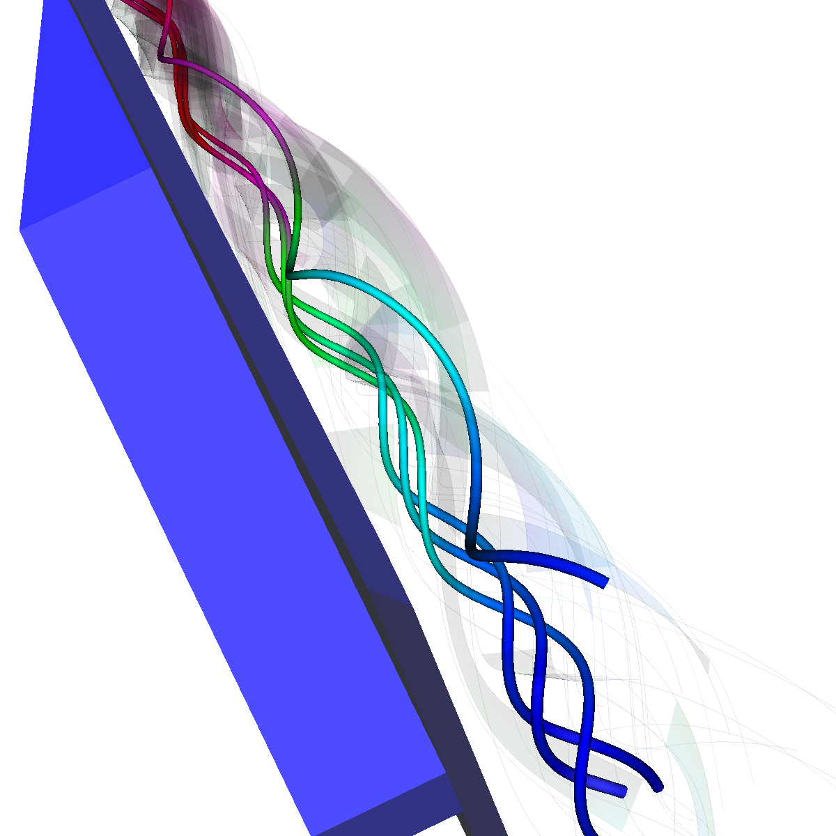 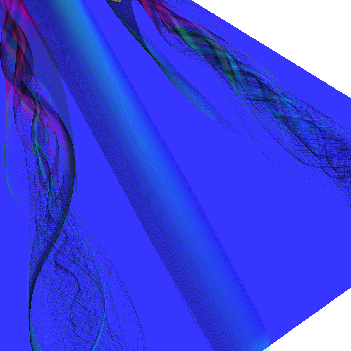 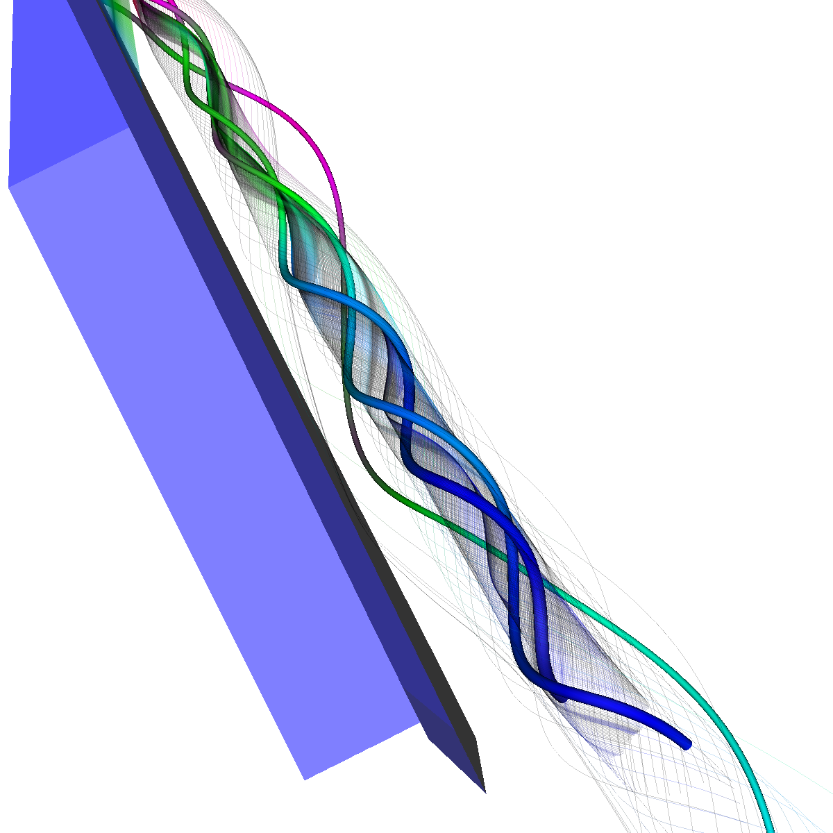 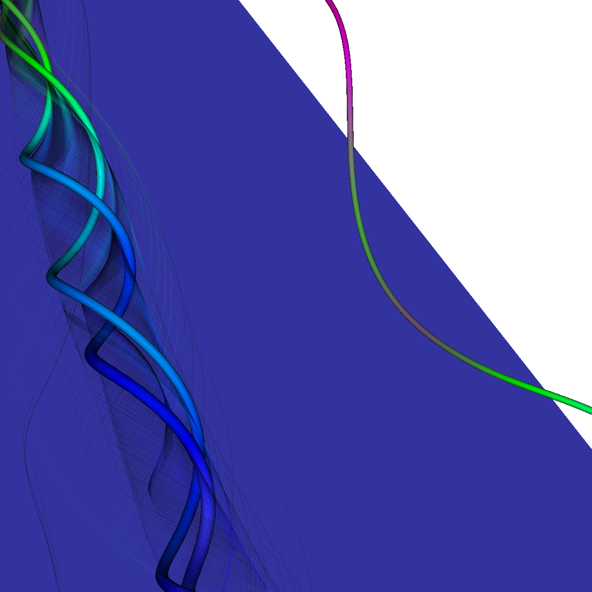 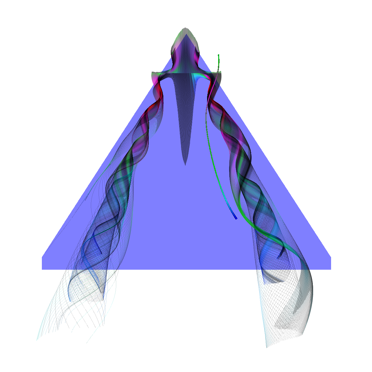 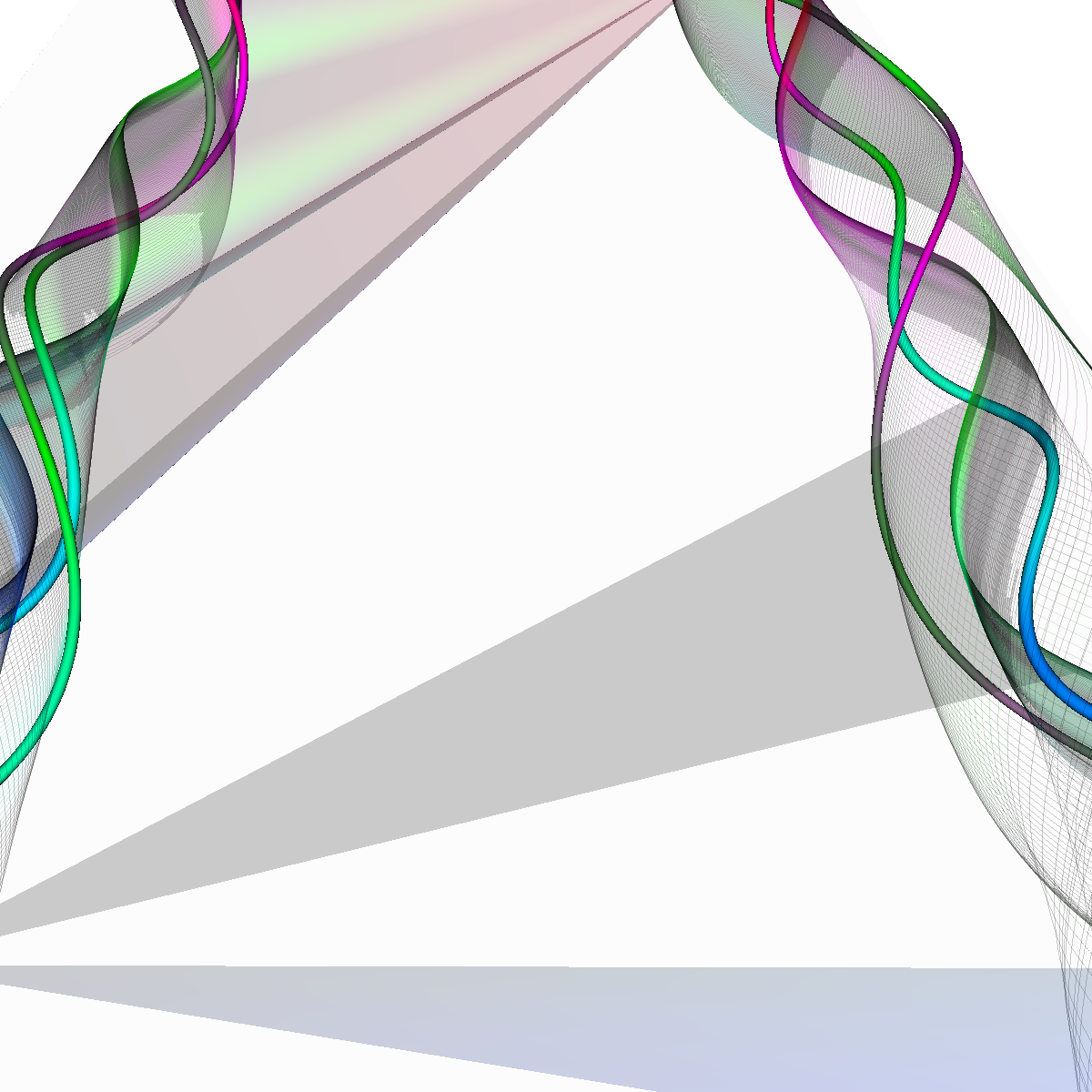 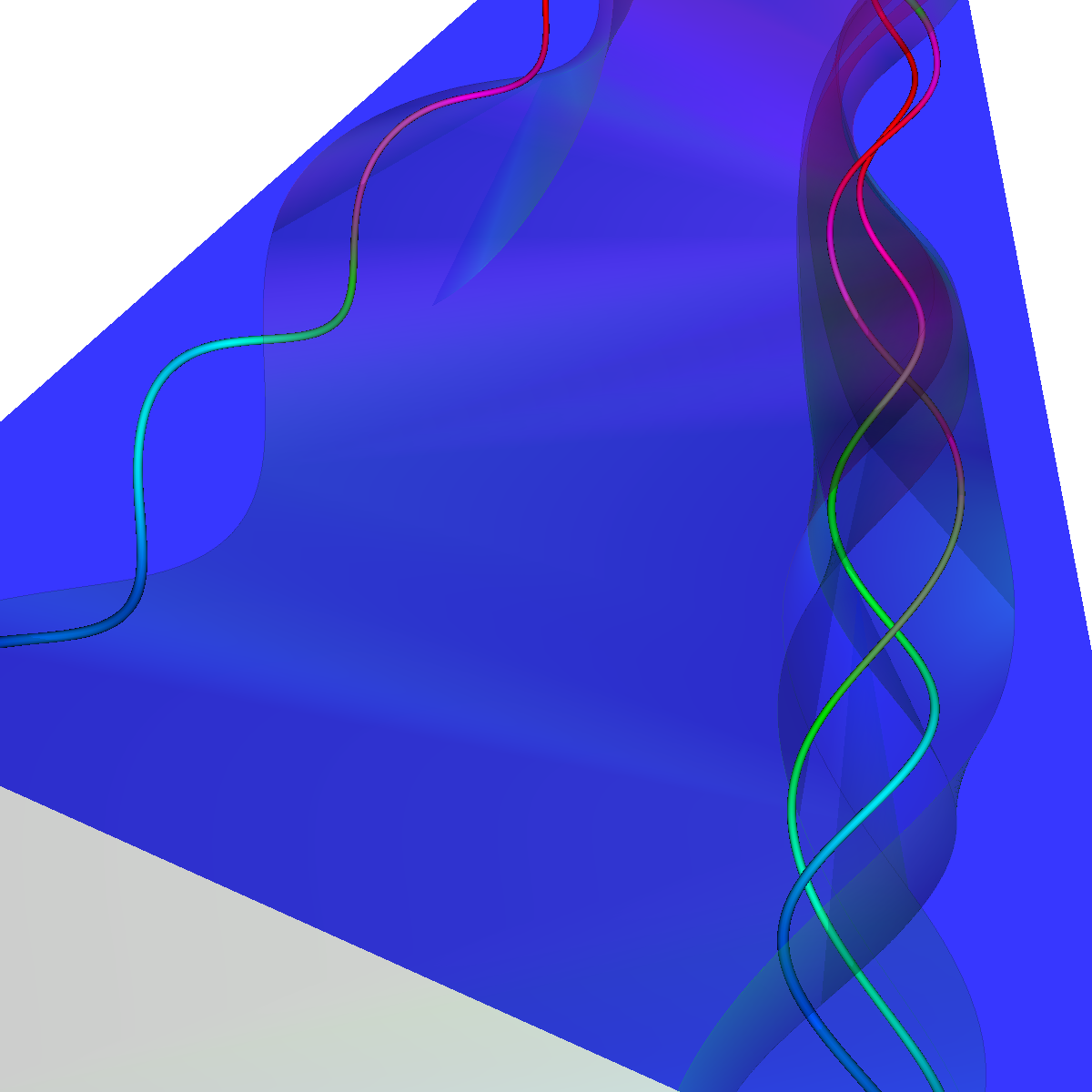 |